Cost function and likelihood
Cost function
The cost function that is minimized in the optimization performed during CA is described here. The cost is reported in the result tables after running CA, as individual cost in the table of individual parameters, and as total cost in a separate table, together with the likelihood and additional criteria.
Formulas for the cost function used in PKanalix are derived in the framework of generalized least squares described in the publication Banks, H. T., & Joyner, M. L. (2017). AIC under the framework of least squares estimation. Applied Mathematics Letters, 74, 33-45, with an additional scaling to put the same weight on different observation types.
The total cost function, shown in the COST table in the results, is a sum of individual cost per each occasion (sum over id-occ):
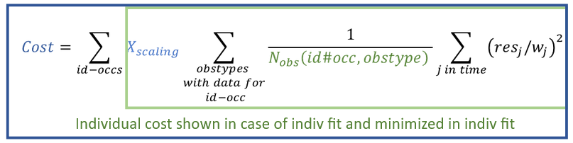
where in the above formula:
- \( N_{obs}(id\#occ, obsType) \) denotes the number of observations for one individual, one occasion and one observation type (ie one model output mapped to data, eg parent and metabolite, or PK and PD, see here).
- \( res_j = Y_{pred}(t_j) – Y_{obs}(t_j) \) are residuals at measurement times \( t_j \), where \(Y_{pred}\) are the predictions for every time point \(t_j\) , and \(Y_{obs}\) the observations read from the dataset.
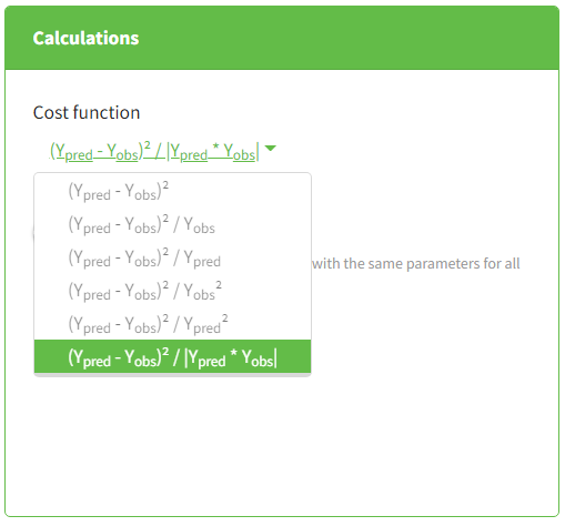
- \( w_j \) are weights \(1, Y_{obs}, Y_{pred}, \sqrt{|Y_{obs}|}, \sqrt{|Y_{pred}|}, \sqrt{|Y_{obs}|\cdot |Y_{pred}|} \) depending on the choice in the CA task > Settings > Calculations, as explained in this tutorial video.
\( X_{scaling} \) is a scaling parameter given by:
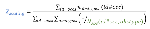
with \( n_{obsTypes}(id\#occ) \) number of observation IDs mapped to a model output for one individual and one occasion. Note that if there is only one observation type (model output mapped to an observation ID), \( X_{scaling} =1\) and the cost function is a simple sum of squares over all observations, weighted by the \(w_j\) .
Likelihood
The likelihood is not directly used for the optimization in CA, but it is possible to derive it based on the optimal cost obtained with the following formula (details in Banks et al):
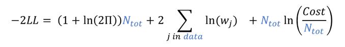
where
- -2LL stands for -2 x ln(Likelihood)
- \( N_{tot} \) is the total number of observations for all individuals, all occasions and all mapped model outputs
- \(w_j\) are the weights as defined above
Additional Criteria
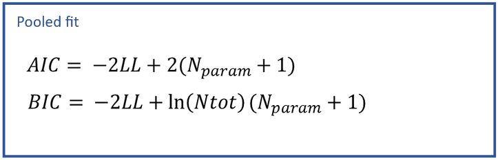
Additional information criteria are the Akaike Information Criteria (AIC) and the Bayesian Information Criteria (BIC). They are used to compare models. They penalize -2LL by the number of model parameters used for the optimization \( N_{param} \), and the number of observations: \( N_{tot} \), total number of observations, and \(N_{obs}(id\#occ)\), number of observations for every subject-occasion. This penalization enables to compare models with different levels of complexity. Indeed, with more parameters, a model can easily give a better fit (lower -2LL), but with too many parameters, a model loses predictive power and confidence in the parameter estimates. If not only the -2LL, but also AIC and BIC criteria decrease after changing a model, it means that the increased likelihood is worth increasing the model complexity.
This formula simplifies if the “pooled fit” option is selected in the calculation settings of the CA task:
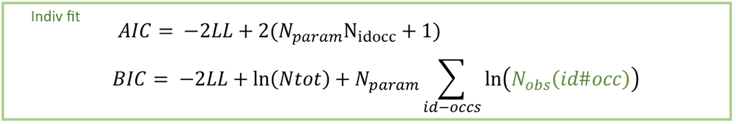
AIC derivation in the case of individual fits
The total AIC for all individuals penalizes -2LL with 2x the number of parameters used in the optimization. For the structural model, we use \(N_{param} N_{id\#occ}\), where \(N_{param}\) is the number of parameters in the structural model and \(N_{id\#occ}\) is the number of subject-occasions (since there is a set of parameters of each id#occ). For the statistical model, we also calculate implicitly one parameter \(\sigma^2\), which is the variance of the residual error model shared by all the individuals (it is derived using the sum of squares of residuals as described in Banks et al). Therefore, AIC penalizes -2LL by \(2(N_{param} N_{idocc} + 1)\).
BIC derivation in the case of individual fits
The total BIC should penalize -2LL by (nb of parameters) x ln(nb of data points). In this case, we should distinguish between the data for each id#occ, which is used to optimize Nparam parameters, and the data for all individuals, which is used all together to calculate the residual variance σ². To penalize each individual’s data in the optimization with Nparam, we add the term \(N_{param} \times ln(N_{obs}(id\#occ))\) for each id#occ. To penalize the calculation of the error model parameter with all the observations (substitution of \(\sigma\) as described in Banks et al), we add the term \(1\times ln(N_{tot})\).