The dataset format that is used in PKanalix is the same as for the entire MonolixSuite, to allow smooth transitions between applications. In this format, some rules have to be fullfilled, for example:
- Each line corresponds to one individual and one time point.
- Each line can include a single measurement (also called observation), or a dose amount (or both a measurement and a dose amount).
- Dose amount should be indicated for each individual dose in a column AMOUNT, even if it is identical for all.
- Headers are free but there can be only one header line.
If your dataset is not in this format, in most cases, it is possible to format it in a few steps in the data formatting tab, to incorporate the missing information.
In this case, the original dataset should be loaded in the “Format data” box, or directly in the “Data Formatting” tab, instead of the “Data” tab. In the data formatting module, you will be guided to build a dataset in the MonolixSuite format, starting from the loaded csv file. The resulting formatted dataset is then loaded in the Data tab as if you loaded an already-formatted dataset in “Data” directly. Then as for defining any dataset, you can tag columns, accept the dataset, and once accepted, units can be specified in the Data tab and the Filters tab can be used to select only parts of this dataset for analysis. Note that units and filters are neither information to be included in the data file, nor part of the data formatting process.
From the version 2024R1, it is possible to save and reapply data formatting steps on multiple projects, using data formatting presets.
Jump to:
- Data formatting workflow
- Dataset initialization (mandatory step)
- Selecting header lines or lines to exclude to merge header lines or exclude a line
- Tagging mandatory columns such as ID and TIME
- Initialization example Demo project CreateOcc_AdmIdbyCategory.pkx
- Creating occasions from a SORT column to distinguish different sets of measurements within each subject, (eg formulations). Demo project CreateOcc_AdmIdbyCategory.pkx
- Selecting an observation type (required to add a treatment)
- Merging observations from several columns
- As observation ids to map them to several outputs in CA. Demo project merge_obsID_ParentMetabolite.pkx
- As occasions to analyze them simultaneously in NCA. Demo project merge_occ_ParentMetabolite.pkx
- Option “Duplicate information from undefined columns”
- Specifying censoring from censoring tags eg “BLQ” instead of a number in an observation column. Demo project DoseAndLOQ_manual.pkx
- Adding doses in the dataset Demo project DoseAndLOQ_manual.pkx
- Reading censoring limits or dosing information from the dataset “by category” or “from data”. Demo projects DoseAndLOQ_byCategory.pkx and DoseAndLOQ_fromData.pkx
- Creating occasions from dosing intervals to analyze separately the measurements following different doses.Demo project doseIntervals_as_Occ.mlxtran
- Handling urine data to merge start and end times in a single column. Demo project Urine_LOQinObs.pkx
- Adding new columns from an external file, eg new covariates, or individual parameters estimated in a previous analysis. Demo warfarin_PKPDseq_project.mlxtran
- Exporting the formatted dataset
1. Data formatting workflow
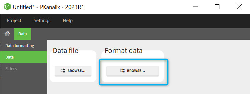
When opening a new project, two Browse buttons appear. The first one, under “Data file”, can be used to load a dataset already in a MonolixSuite-standard format, while the second one, under “Format data”, allows to load a dataset to format in the Data formatting module.
After loading a dataset to format, data formatting operations can be specified in several subtabs: Initialization, Observations, Treatments and Additional columns.
- Initialization is mandatory and must be filled before using the other subtabs.
- Observations is required to enable the Treatments tab.
After Initialization has been validated by clicking on “Next”, a button “Preview” is available from any subtab to view in the Data tab the formatted dataset based on the formatting operations currently specified.

2. Dataset initialization
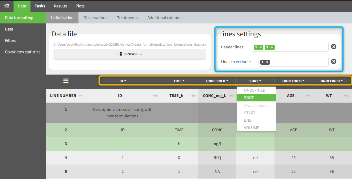
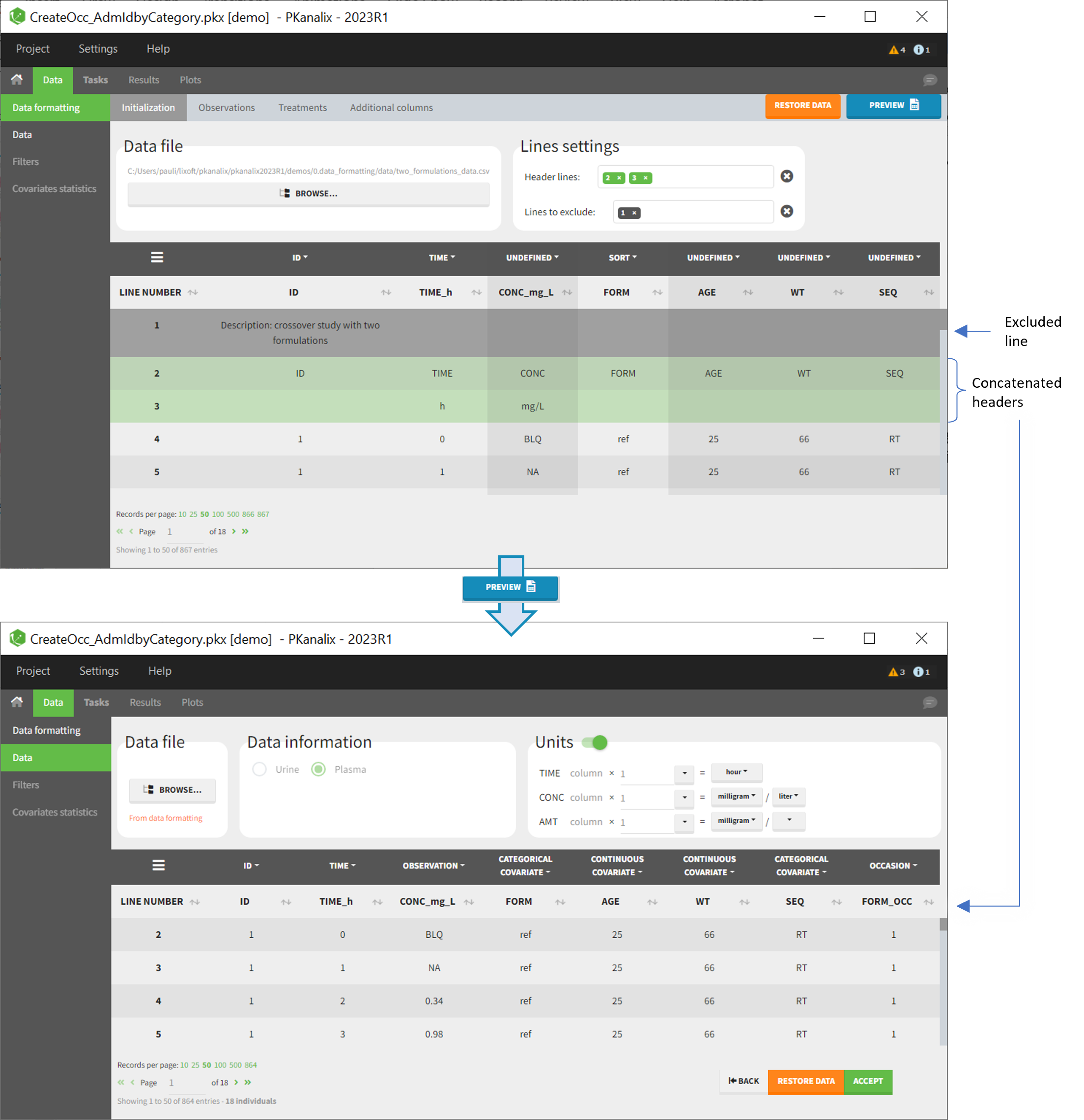
The first tab in Data formatting is named Initialization. This is where the user can select header lines or lines to exclude (in the blue area on the screenshot below) or tag columns (in the yellow area).
Selecting header lines or lines to exclude
These settings should contain line numbers for lines that should be either handled as column headers or that should be excluded.
- Header lines: one or several lines containing column header information. By default, the first line of the dataset is selected as header. If several lines are selected, they are merged by data formatting into a single line, concatenating the cells in each column.
- Lines to exclude (optional): lines that should be excluded from the formatted dataset by data formatting.
Tagging mandatory columns
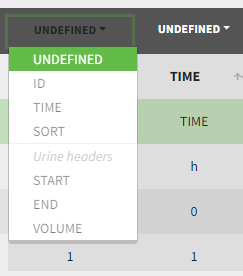
Only the columns corresponding to the following tabs must be tagged in Initialization, while all the other columns should keep the default UNDEFINED tag:
- ID (mandatory): subject identifiers
- TIME (mandatory): the single time column
- SORT (optional): one or several columns containing SORT variables can be tagged as SORT. Occasions based on these columns will be created in the formatted dataset as described in Section 3.
- START, END and VOLUME (mandatory in case of urine data): these column tags replace the TIME tag in case of urine data, if the urine collection time intervals are encoded in the dataset with two time columns for the start and end times of the intervals. In that case there should also be a column with the urine volume in each interval. See Section 10 for more details.
Initialization example
- demo CreateOcc_AdmIdbyCategory.pkx (the screenshot below focuses on the formatting initialization and excludes other elements present in the demo):
In this demo the first line of the dataset is excluded because it contains a description of the study. The second line contains column headers while the third line contains column units. Since the MonolixSuite-standard format allows only a single header line, lines 2 and 3 are merged together in the formatted dataset.
3. Creating occasions from a SORT column
A SORT variable can be used to distinguish different sets of measurements (usually concentrations) within each subject, that should be analyzed separately by PKanalix (for example: different formulations given to each individual at different periods of time, or multiple doses where concentration profiles are available to be analyzed following several doses).
In PKanalix, these different sets of measurements must be distinguished as OCCASIONS (or periods of time), via the OCCASION column-type. However, a column tagged as OCCASION can only contain integers with occasion indexes. Thus, if a column with a SORT variable contains strings, its format must be adapted by Data formatting, in the following way:
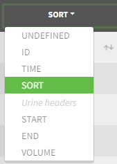
- the user must tag the column as SORT in the Initialization subtab of Data formatting,
- the user validates the Initialization with “Next”, then clicks on “Preview” (after optionally defining other data formatting operations),
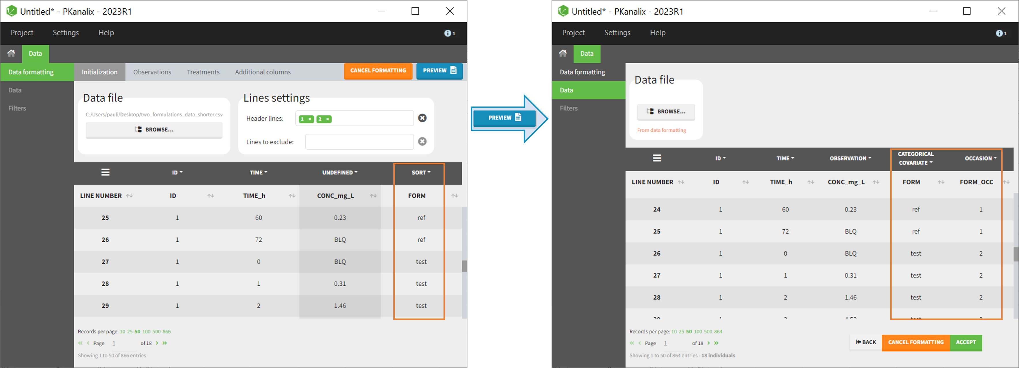
- the formatted data is shown in Data: the column tagged as SORT is automatically duplicated. The original column is automatically tagged as CATEGORICAL COVARIATE in Data, while the duplicated column, which has the same name appended with “_OCC”, is tagged as OCCASION. This column contains occasion indexes instead of strings.
Example:
- demo CreateOcc_AdmIdbyCategory.pkx (the screenshot below focuses on the formatting of occasions and excludes other elements present in the demo):
The image below shows lines 25 to 29 from the dataset from the CreateOcc_AdmIdbyCategory.pkx demo, where covariate columns have been removed to simplify the example. This dataset contains two sets of concentration measurements for each individual, corresponding to two different drug formulations administered on different periods. The sets of concentrations are distinguished with the FORM column, which contains “ref” and “test” categories (reference/test formulations). The column is tagged as SORT in Data formatting Initialization. After clicking on “Preview”, we can see in the Data tab that a new column named FORM_OCC has been created with occasion indexes for each individual: for subject 1, FORM_OCC=1 corresponds to the reference formulation because it appears first in the dataset, and FORM_OCC=2 corresponds to the test formulation because it appears in second in the dataset.
4. Selecting an observation type
The second subtab in Data formatting allows to select one or several observation types. An observation type corresponds to a column of the dataset, that contains a type of measurements (usually drug concentrations, but it can also be PD measurements for example). Only columns that have not been tagged as ID, TIME or SORT are available as observation type.
This action is optional and can have several purposes:
- If doses must be added by Data formatting (see Section 7), specifying the column containing observations is mandatory, to avoid duplicating observations on new dose lines.
- If several observation types exist in different columns (for example: concentrations for different analytes, or measurements for PK and PD), they must be specified in Data formatting to be merged into a single observation column (see Section 5).
- In the MonolixSuite-standard format, the column containing observations can only contain numbers, and no string except “.” for a missing observation. Thus if this column contains strings in the original dataset, it must be adapted by Data formatting, with two different cases:
- if the strings are tags for censored observations (usually BLQ: below the limit of quantification), they can be specified in Data formatting to adapt the encoding of the censored observations (see Section 6),
- any other string in the column is automatically replaced by “.” by Data formatting.
5. Merging observations from several columns
The MonolixSuite-standard format allows a single column containing all observations (such as concentrations or PD measurements). Thus if a dataset contains several observation types in different columns (for example: concentrations for different analytes, or measurements for PK and PD), they must be specified in Data formatting to be merged into a single observation column.
In that case, different settings can be chosen in the area marked in orange in the screenshot below:
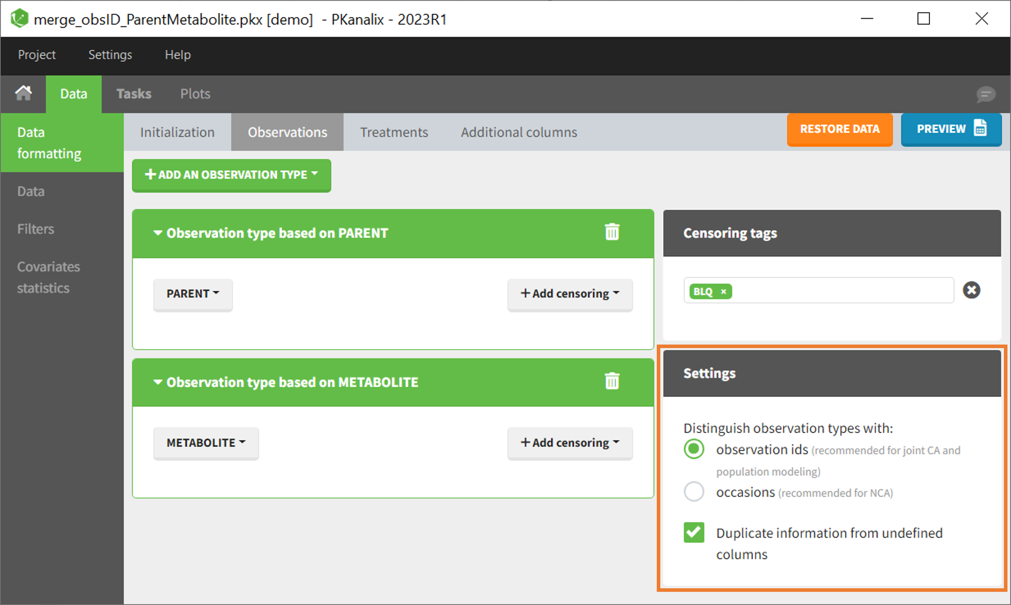
- The user must choose between distinguishing observation types with observation ids or occasions.
- The user can unselect the option “Duplicate information from undefined columns”.
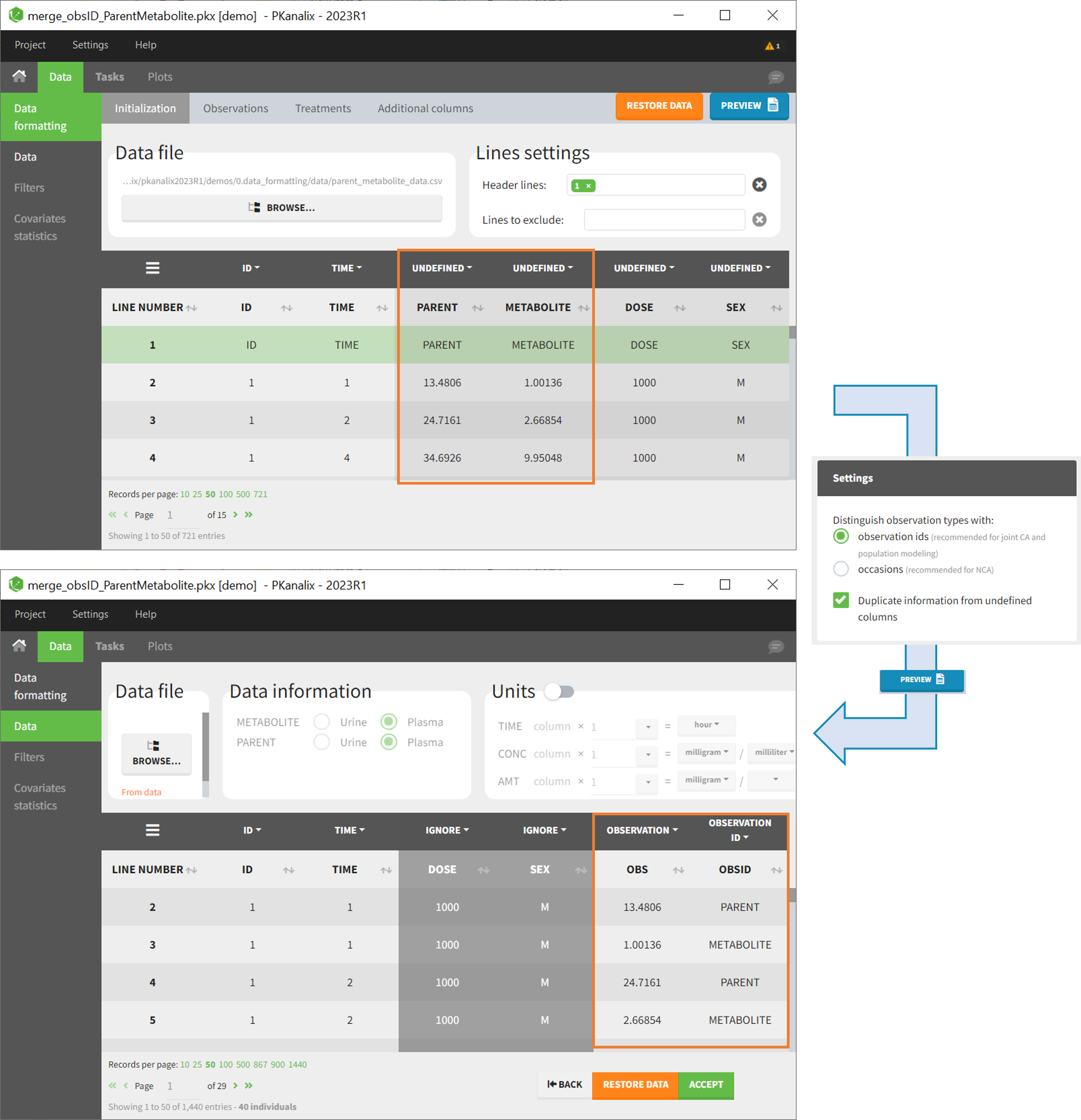
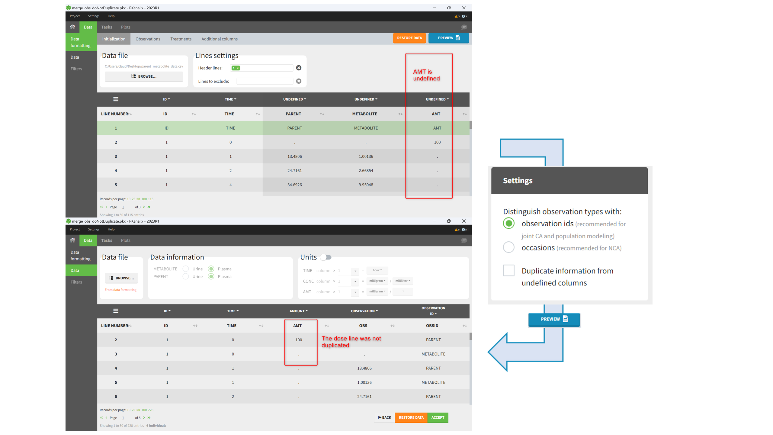
As observation ids
After selecting the “Distinguish observation types with: observation ids” option and clicking “Preview,” the columns for different observation types are combined into a single column called “OBS.” Each row of the dataset is duplicated for each observation type, with one value per observation type. Additionally, an “OBSID” column is created, with the name of the observation type corresponding to the measurement on each row.
This option is recommended for joint modeling of observation types, such as CA in PKanalix or population modeling in Monolix. It is important to note that NCA cannot be performed on two different observation ids simultaneously, so it is necessary to choose one observation id for the analysis.
Example:
- demo merge_obsID_ParentMetabolite.pkx (the screenshot below focuses on the formatting of observations and excludes other elements present in the demo):
This demo involves two columns that contain drug parent and metabolite concentrations. When merging both observation types with observation ids, a new column called OBSID is generated with categories labeled as “PARENT” and “METABOLITE.”
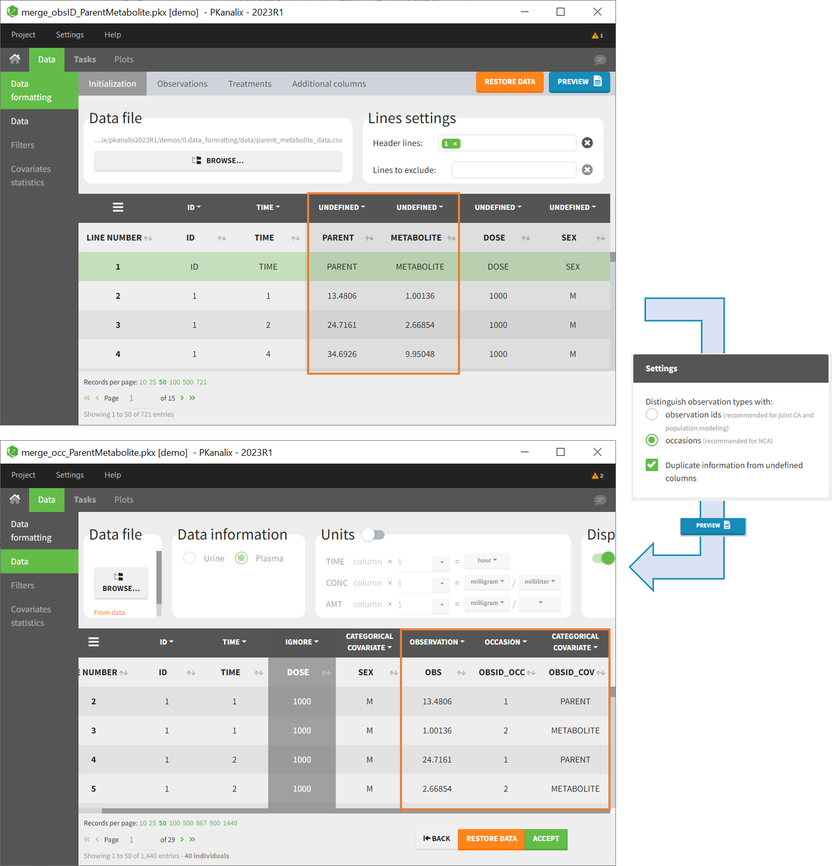
As occasions
After selecting the “Distinguish observation types with: occasions” option and clicking “Preview,” the columns for different observation types are combined into a single column called “OBS.” Each row of the dataset is duplicated for each observation type, with one value per observation type. Additionally, two columns are created: an “OBSID_OCC” column with the index of the observation type corresponding to the measurement on each row, and an “OBSID_COV” with the name of the observation type.
This option is recommended for NCA, which can be run on different occasions for each individual. However, joint modeling of the observation types with CA or population modeling with Monolix cannot be performed with this option.
Example:
- demo merge_occ_ParentMetabolite.pkx:
This demo involves two columns that contain drug parent and metabolite concentrations. When merging both observation types with occasions, two new columns called OBSID_OCC and OBSID_COV are generated with OBSID_OCC=1 corresponding to OBSID_COV=”PARENT” catand OBSID_OCC=2 corresponding to OBSID_COV=”METABOLITE.”
Duplicate information from undefined columns
When merging two observation columns into a single column, all other columns will see their lines duplicated. The data formatting will know how to treat columns which have been tagged in the Initialization tab, but not the other columns (header “UNDEFINED”) which are not used for data formatting. A checkbox enables to decide if the information from these columns should be duplicated on the new lines, or if “.” should be used instead. The default option is to duplicate information, because in general, the undefined columns correspond to covariates with one value per individual, so this value is the same for the two lines that correspond to the same id.
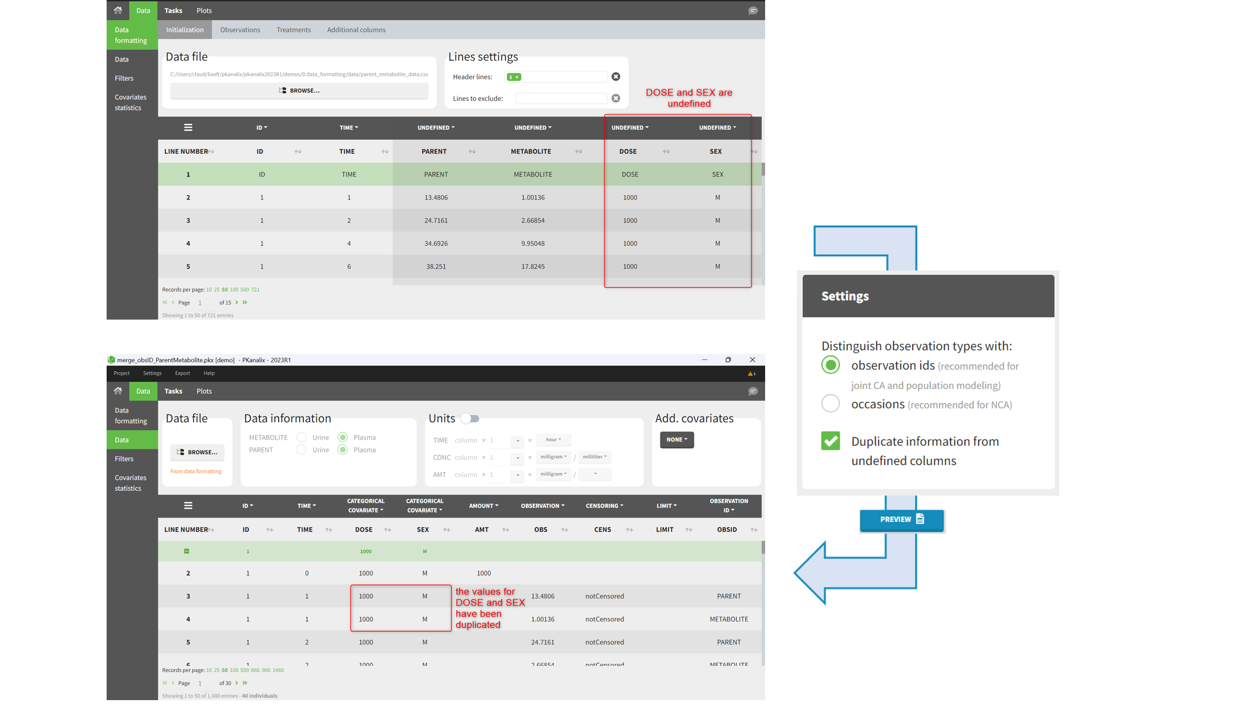
It is rare that you need to uncheck this box. An example where you should not duplicate the information is if you already have a column Amount in the MonolixSuite format, so with a dose amount only at the dosing time, and “.” everywhere else. If you do not want to specify amount again in data formatting, and simply want to merge observation columns as observation ids, you should not duplicate the lines of the Amount column which is undefined. Indeed, the dose amounts have been administered only once.
6. Specifying censoring from censoring tags
In the MonolixSuite-standard format, censored observations are encoded with a 1or -1 flag in a column tagged as CENSORING in the Data tab, while exact observations have a 0 flag in that column. In addition, on rows for censored observations, the LOQ is indicated in the observation column: it is the LLOQ (lower limit of quantification) if CENSORING=1 or the ULOQ (upper limit of quantification) if CENSORING=-1. Finally, to specify a censoring interval, an additional column tagged as LIMIT in the Data tab must exist in the dataset, with the other censoring bound.
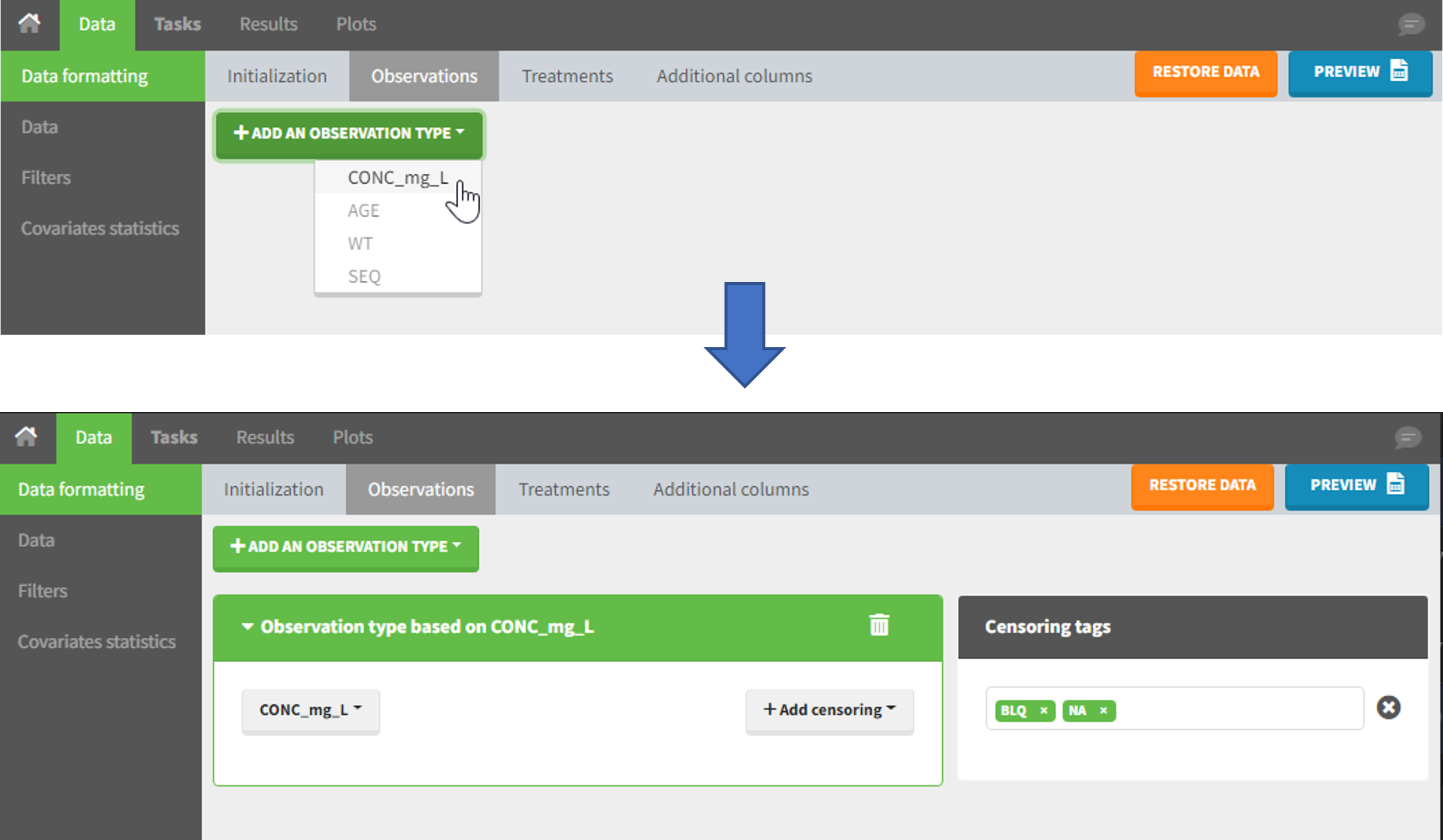
The Data Formatting module can take as input a dataset with censoring tags directly in the observation column, and adapt the dataset format as described above. After selecting one or several observation types in the Observations subtab (see Section 4), all strings found in the corresponding columns are displayed in the “Censoring tags” on the right of the observation types. If at least one string is found, the user can then define some censoring associated with an observation type and with one or several censoring tags with the button “Add censoring”. Additionally, option “Use all automatically detected tags” exist and can be used when all censoring tags correspond to the same censoring type (this option is recommended for the usage with data formatting presets, if censoring tags vary between data sets in which the preset will be used). 3 types of censoring can be defined:
- LLOQ: this corresponds to left-censoring, where the censored observation is below a lower limit of quantification (LLOQ), that must specified by the user. In that case Data Formatting replaces the censoring tags in the observation column by the LLOQ, and creates a new CENS column tagged as CENSORING in the Data tab, with 1 on rows that had censoring tags before formatting, and 0 on other rows.
- ULOQ: this corresponds to right-censoring, where the censored observation is above an upper limit of quantification (ULOQ), that must specified by the user. Here Data Formatting replaces the censoring tags in the observation column by the ULOQ, and creates a new CENS column tagged as CENSORING in the Data tab, with -1 on rows that had censoring tags before formatting, and 0 on other rows.
- Interval: this is for interval-censoring, where the user must specify two bound of a censoring interval, to which the censored observation belong. Data Formatting replaces the censoring tags in the observation column by the upper bound of the interval, and creates two new columns: a CENS column tagged as CENSORING in the Data tab, with 1 on rows that had censoring tags before formatting, and 0 on other rows, and a LIMIT column with the lower bound of the censoring interval on rows that had censoring tags before formatting, and “.” on other rows.
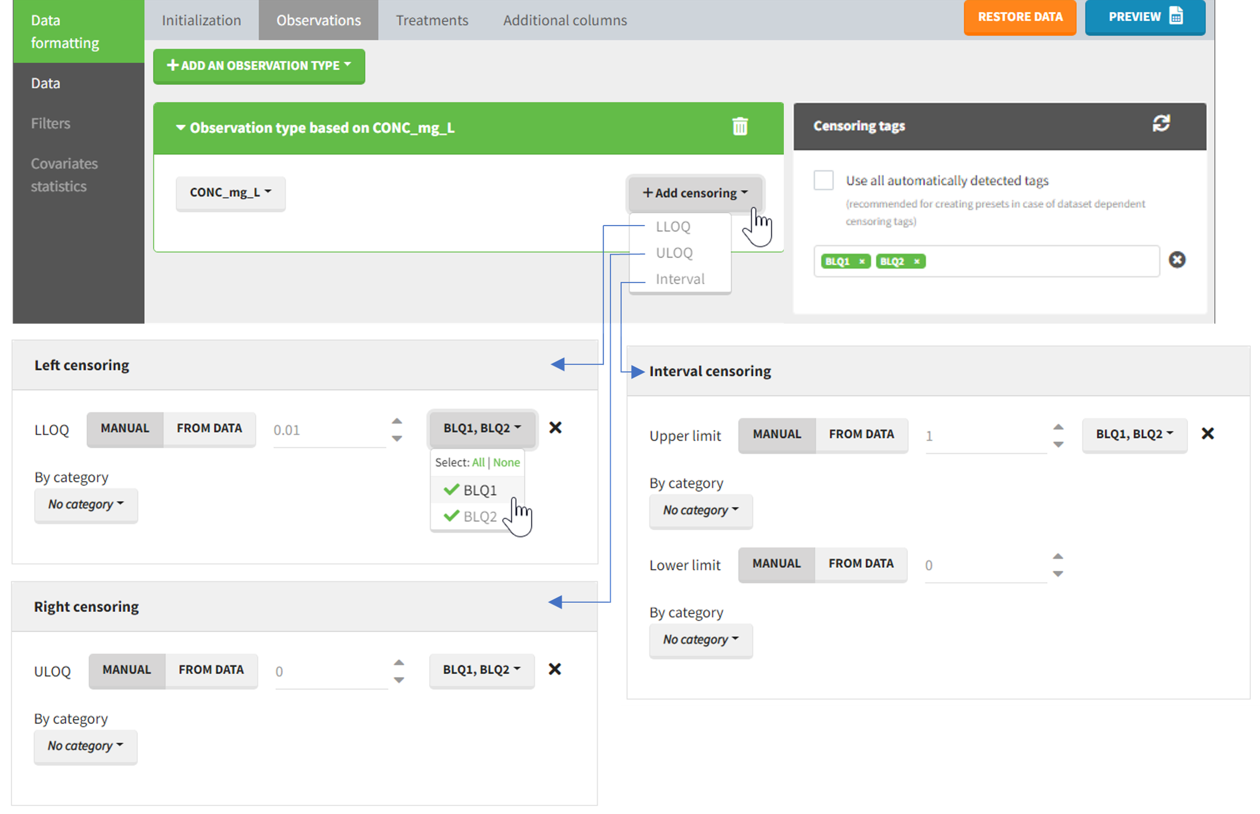
For each type of censoring, available options to define the limits are:
- “Manual“: limits are defined manually, by entering the limit values for all censored observations.
- “By category“: limits are defined manually for different categories read from the dataset.
- “From data“: limits are directly read from the dataset.
The options “by category” and “from data” are described in detail in Section 8.
Example:
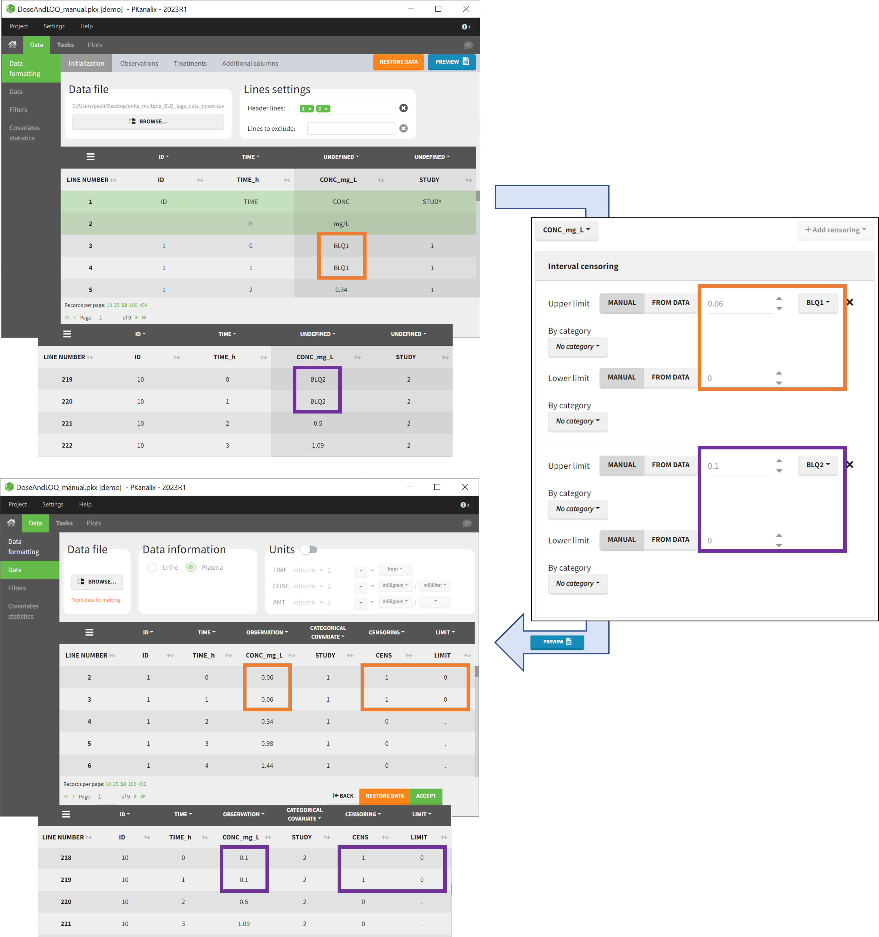
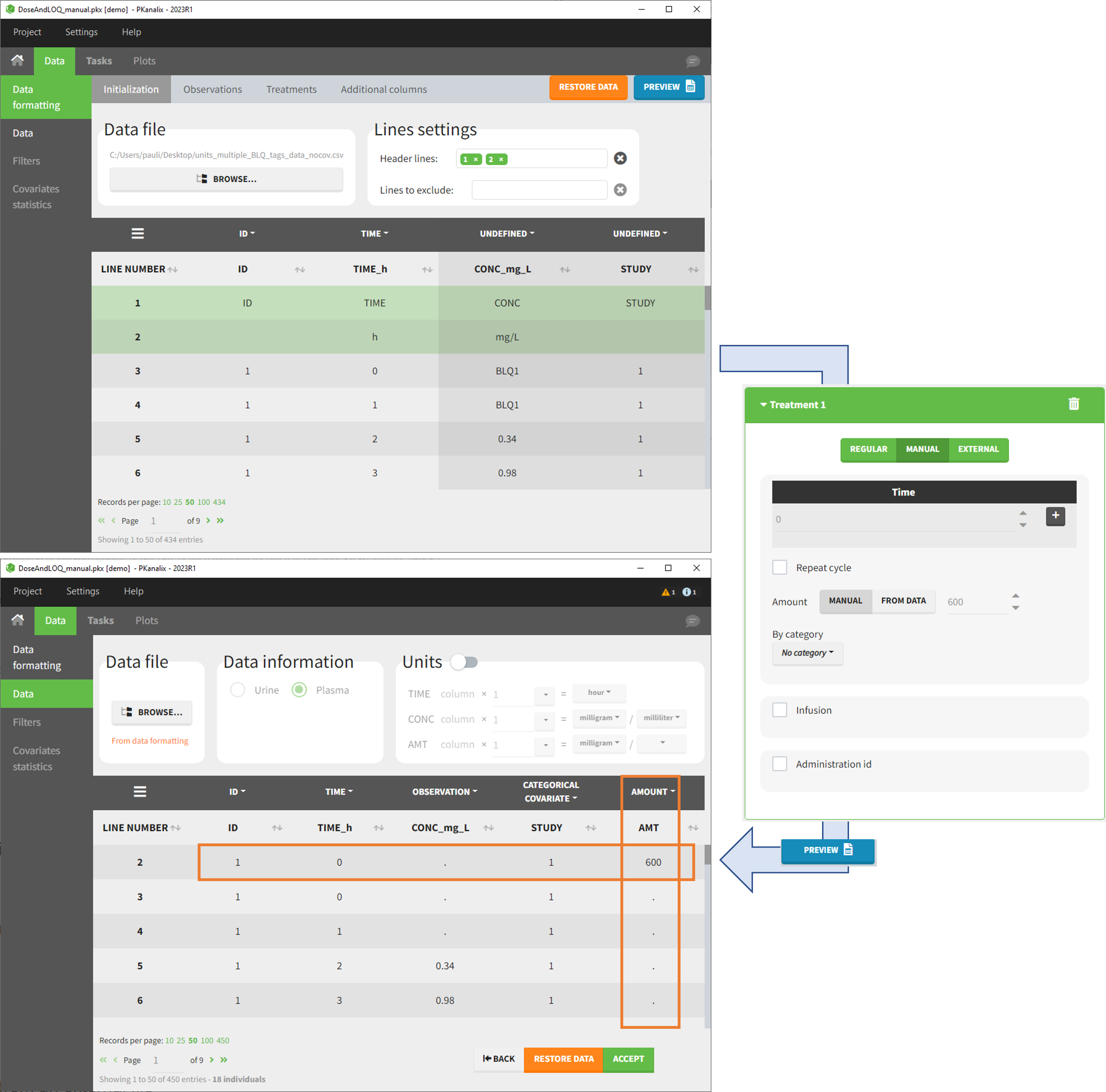
- demo DoseAndLOQ_manual.pkx (the screenshot below focuses on the formatting of censored observations and excludes other elements present in the demo):
In this demo there are two censoring tags in the CONC column: BLQ1 (from Study 1) and BLQ2 (from Study 2), that correspond to different LLOQs. An interval censoring is defined for each censoring tag, with manual limits, where LLOQ=0.06 for BLQ1 and LLOQ=0.1 for BLQ2, and the lower limit of the censoring interval being 0 in both cases.
7. Adding doses in the dataset
Datasets in MonolixSuite-standard format should contain all information on doses, as dose lines. An AMOUNT column records the amount of the administrated doses on dose-lines, with “.” on response-lines. In case of infusion, an INFUSION DURATION or INFUSION RATE column records the infusion duration or rate. If there are several types of administration, an ADMINISTRATION ID column can distinguish the different types of doses with integers.
If doses are missing from a dataset, the Data Formatting module can be used to add dose lines and dose-related columns: after initializing the dataset, the user can specify one or several treatments in the Treatments subtab. The following operations are then performed by Data Formatting:
- a new dose line is inserted in the dataset for each defined dose, with the dataset sorted by subject and times. On such a dose line, the values from the next line are duplicated for all columns, except for the observation column in which “.” is used for the dose line.
- A new column AMT is created with “.” on all lines except on dose lines, on which dose amounts are used. The AMT column is automatically tagged as AMOUNT in the Data tab.
- If administration ids have been defined in the treatment, an ADMID column is created, with “.” on all lines except on dose lines, on which administration ids are used. The ADMID column is automatically tagged as ADMINISTRATION ID in the Data tab.
- If an infusion duration or rate has been defined, a new INFDUR (for infusion duration) or INFRATE (for infusion rate) is created, with “.” on all lines except on dose lines. The INFDUR column is automatically tagged as INFUSION DURATION in the Data tab, and the INFRATE column is automatically tagged as INFUSION RATE.
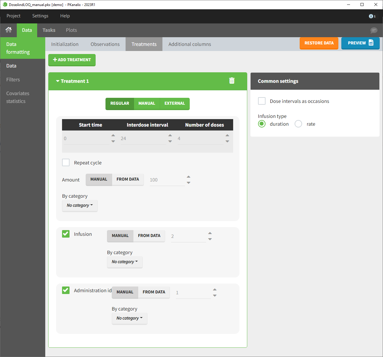
For each treatment, the dosing schedule can defined as:
- regular: for regularly spaced dosing times, defined with the start time, inter-dose internal, and number of doses. A “repeat cycle” option allows to repeat the regular dosing schedule to generate a more complex regimen.
- manual: a vector of one or several dosing times, each defined manually. A “repeat cycle” option allows to repeat the manual dosing schedule to generate a more complex regimen.
- external: an external text file with columns id (optional), occasions (optional), time (mandatory), amount (mandatory), admid (administration id, optional), tinf or rate (optional), that allows to define individual doses.
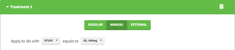
Starting from the 2024R1 version, different dosing schedules can be defined for different individuals, based on information from other columns, which can be useful in cases when different cohorts received different dosing regimens, or when working with data pooled from multiple studies. To define a treatment just for a specific cohort or study, the dropdown on the top of the treatment section can be used:
While dose amounts, administration ids and infusion durations or rates are defined in the external file for external treatments, available options to define them for treatments of type “manual” or “regular” are:
- “Manual“: this applies the same amount (or administration id or infusion duration or rate) to all doses.
- “By category“: dose amounts (or administration id or infusion duration or rate) are defined manually for different categories read from the dataset.
- “From data“: dose amounts (or administration id or infusion duration or rate) are directly read from the dataset.
The options “by category” and “from data” are described in detail in Section 8.
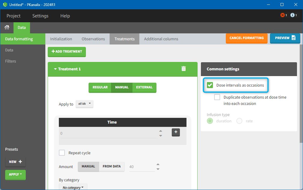
There is a “common settings” panel on the right:
- dose intervals as occasions: this creates a column to distinguish the dose intervals as different occasions (see Section 9).
- infusion type: If several treatments correspond to infusion administration, they need to share the same type of encoding for infusion information: as infusion duration or as infusion rate.
Example:
- demo DoseAndLOQ_manual.pkx (the screenshot below focuses on the formatting of doses and excludes other elements present in the demo):
In this demo, doses are initially not included in the dataset to format. A single dose at time 0 with an amount of 600 is added for each individual by Data Formatting. This creates a new AMT column in the formatted dataset, tagged as AMOUNT.
8. Reading censoring limits or dosing information from the dataset
When defining censoring limits for observations (see Section 6) or dose amounts, administration ids, infusion duration or rate for treatments (see Section 7), two options allow to define different values for different rows, based on information already present in the dataset: “by category” and “from data”.
By category
It is possible to define manually different censoring limits, dose amounts, administration ids, infusion durations, or rates for different categories within a dataset’s column. After selecting this column in the “By category” drop-down menu, the different modalities in the column are displayed and a value must be manually assigned each modality.
- For censoring limits, the censoring limit used to replace each censoring tag depends on the modality on the same row.
- For doses, the value chosen for the newly created column (AMT for amount, ADMID for administration id, INFDUR for infusion duration, INFRATE for infusion rate) on each new dose line depends on the modality on the first row found in the dataset for the same individual and the same time as the dose, or the next time if there is no line in the initial dataset at that time, or the previous time if no time is found after the dose.
Example:
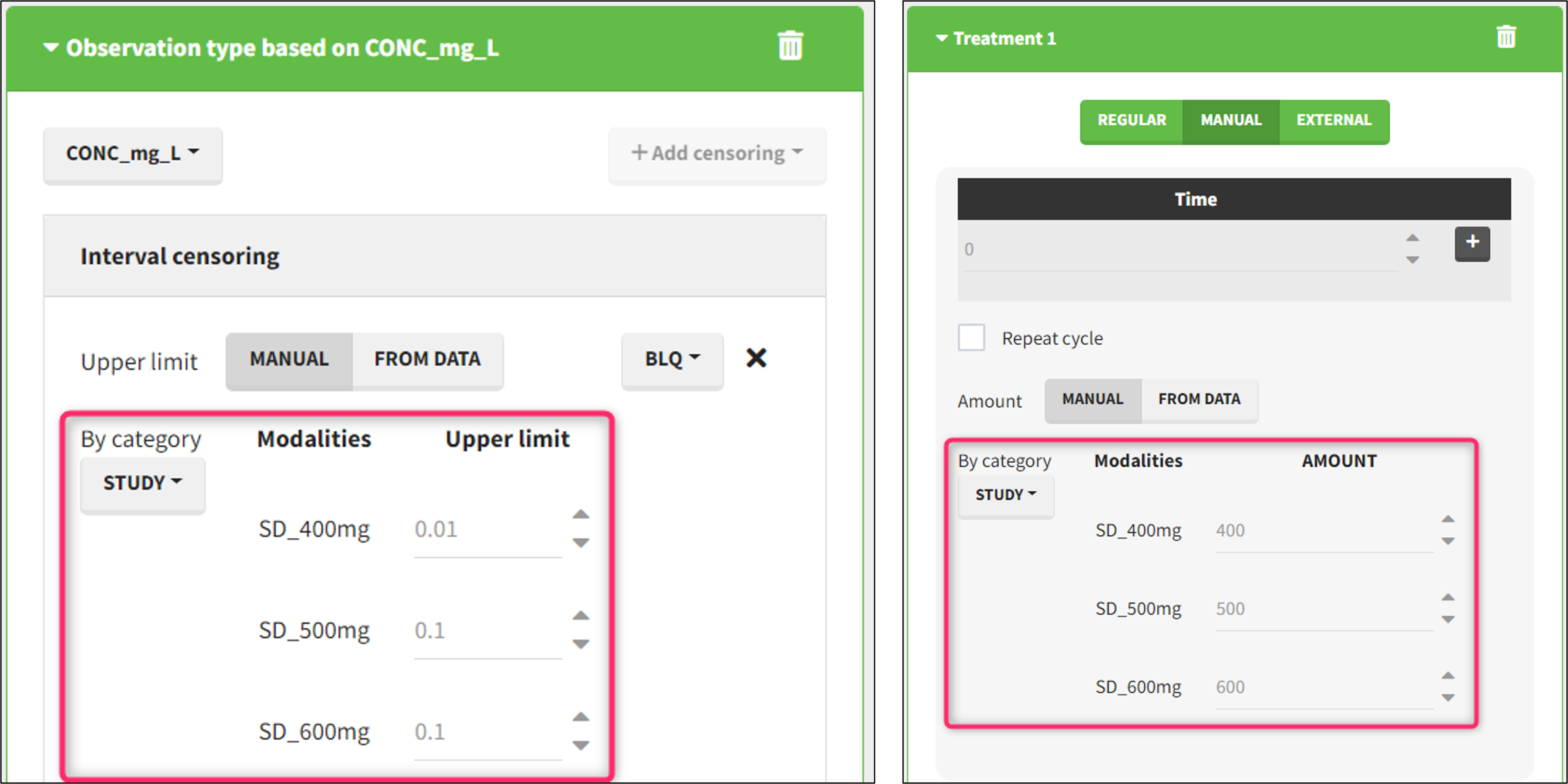
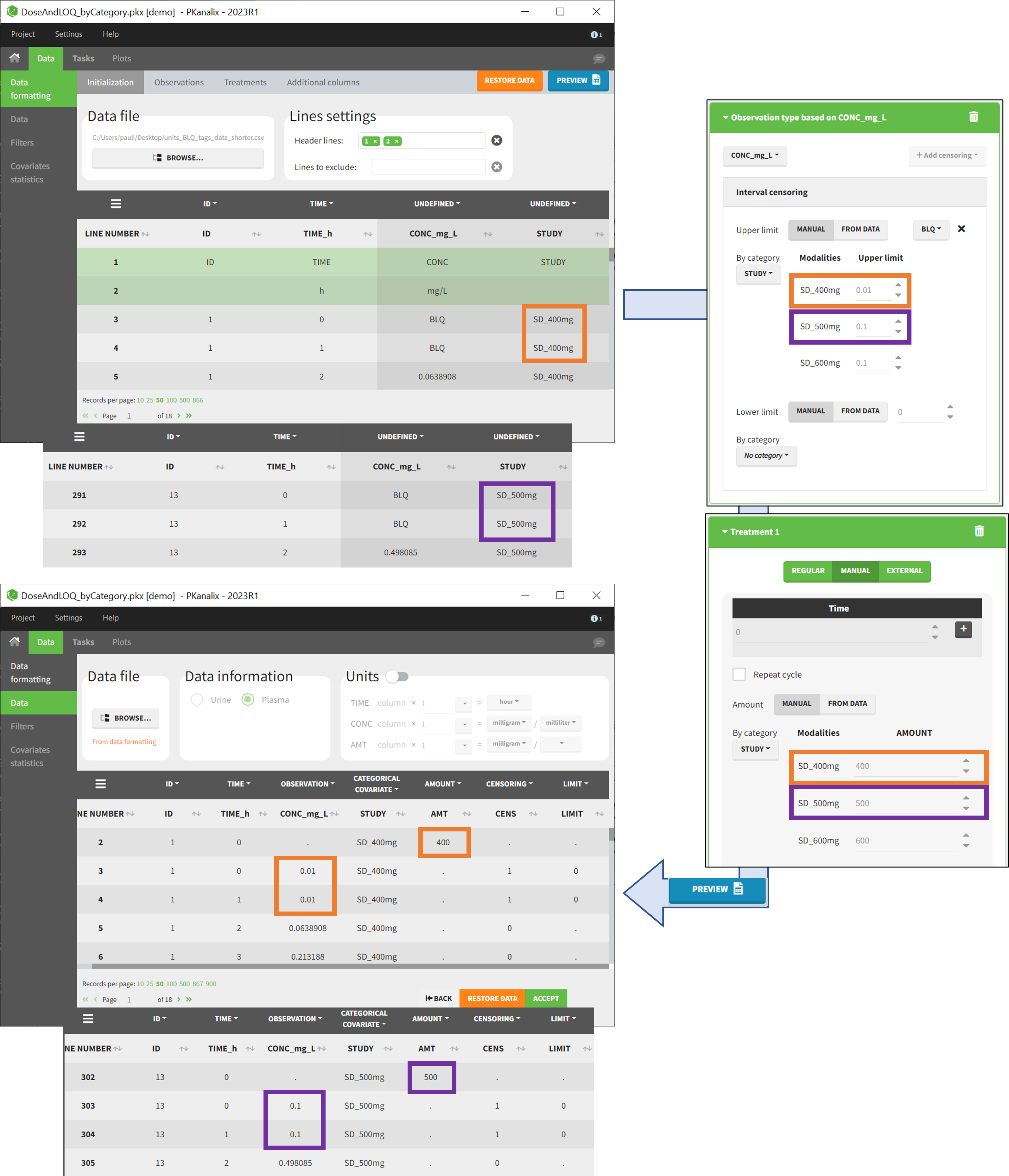
- demo DoseAndLOQ_byCategory.pkx (the screenshot below focuses on the formatting of doses and excludes other elements present in the demo):
In this demo there are three studies distinguished in the STUDY column with the categories “SD_400mg”, “SD_500mg” and “SD_600mg”. In Data Formatting, a single dose is manually defined at time 0 for all individuals, with different amounts depending the STUDY category. In addition, censoring interval is defined for the censoring tags BLQ, with an upper limit of the censoring interval (lower limit of quantification) that also depends on the STUDY category. Three new columns – AMT for dose amounts, CENS for censoring tags (0 or 1), and LIMIT for the lower limit of the censoring intervals – are created by Data Formatting. A new dose line is then inserted at time 0 for each individual.
From data
The option “From data” is used to directly read censoring limits, dose amounts, administration ids, infusion durations, or rates from a dataset’s column. The column must contain either numbers or numbers inside strings. In that case, the first number found in the string is extracted (including decimals with .).
- For censoring limits, the censoring limit used to replace each censoring tag is read from the selected column on the same row.
- For doses, the value chosen for the newly created column (AMT for amount, ADMID for administration id, INFDUR for infusion duration, INFRATE for infusion rate) on each new dose line is read from the selected column on the first row found in the dataset for the same individual and the same time as the dose, or the next time if there is no line in the initial dataset at that time, or the previous time if no time is found after the dose.
Example:
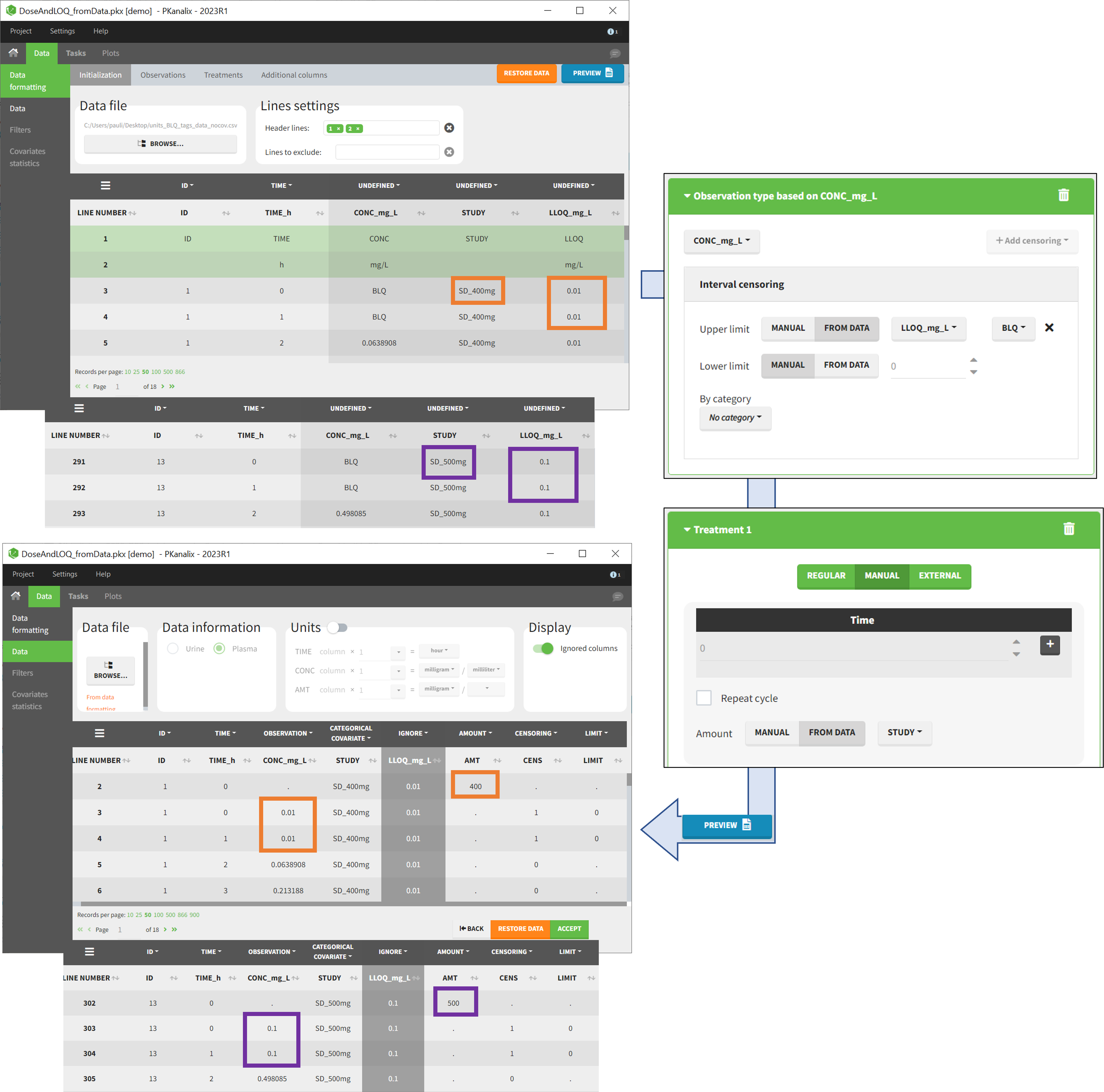
- demo DoseAndLOQ_fromData.pkx (the screenshot below focuses on the formatting of doses and censoring and excludes other elements present in the demo):
In this demo there are three studies distinguished in the STUDY column with the categories “SD_400mg”, “SD_500mg” and “SD_600mg”. In Data Formatting, a single dose is manually defined at time 0 for all individuals, with the amount read the STUDY column. In addition, censoring interval is defined for the censoring tags BLQ, with an upper limit of the censoring interval (lower limit of quantification) read from the LLOQ_mg_L column. Three new columns – AMT for dose amounts, CENS for censoring tags (0 or 1), and LIMIT for the lower limit of the censoring intervals – are created by Data Formatting. A new dose line is then inserted at time 0 for each individual, with amount 400, 500 or 600 for studies SD_400mg, SD_500mg and SD_600mg respectively.
9. Creating occasions from dosing intervals
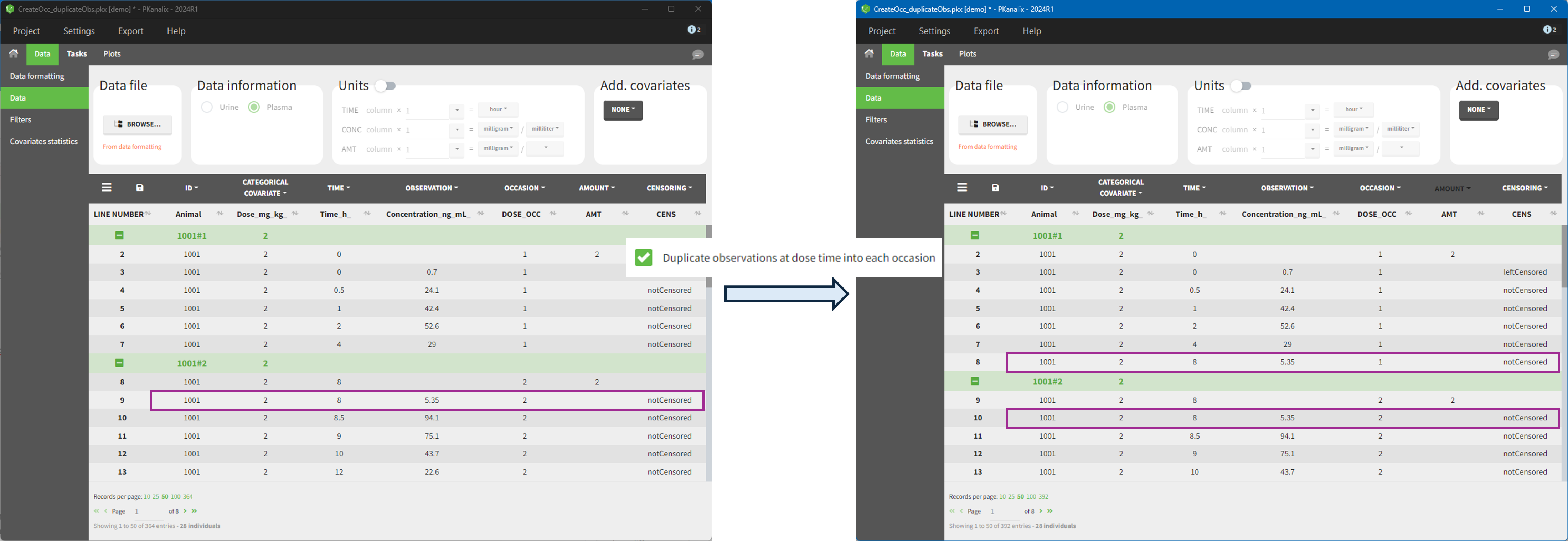
The option “Dose intervals as occasions” in the Treatments subtab of Data Formatting allows to create an occasion column to distinguish dose intervals. This is useful if the sets of measurements following different doses should be analyzed independently for a same individual. From the 2024 version on, an additional option “Duplicate observations at dose times into each occasion” is available. This option allows to duplicate the observations which are at exactly the same time as dose, such that they appear both as last point of the previous occasion and first point of the next occasion.
Example:
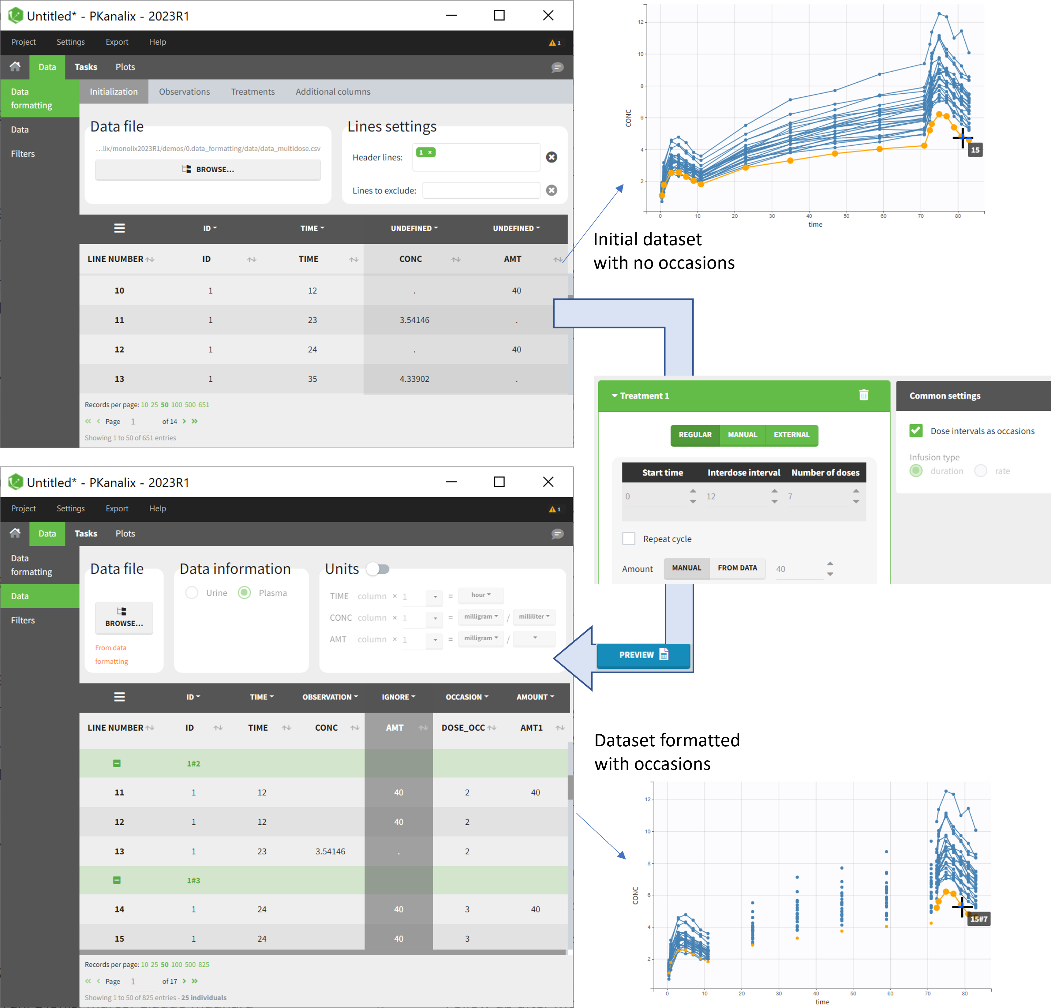
- demo doseIntervals_as_Occ.mlxtran (Monolix demo in the folder 0.data_formatting, here imported into PKanalix):
This demo imported from a Monolix demo has an initial dataset in Monolix-standard format, with multiple doses encoded as dose lines with dose amounts in the AMT column. When using this dataset directly into Monolix or PKanalix, a single analysis is done on each individual concentration profile considering all doses, which means that NCA would be done on the concentrations after the last dose only, and modeling (CA in PKanalix or population modeling in Monolix) would be estimated with a single set of parameter values for each individual. If instead we want to run separate analyses on the sets of concentrations following each dose, we need to distinguish them as occasions with a new column added with the Data Formatting module. To this end, we define the same treatment as in the initial dataset with Data Formatting (here as regular multiple doses) with the option “Dose intervals as occasions” selected. After clicking Preview, Data Formatting adds two new columns: an AMT1 column with the new doses, to be tagged as AMOUNT instead of the AMT column that will now be ignored, and a DOSE_OCC column to be tagged as OCCASION.
Example:
- demo CreateOcc_duplicateObs.pkx:

10. Handling urine data
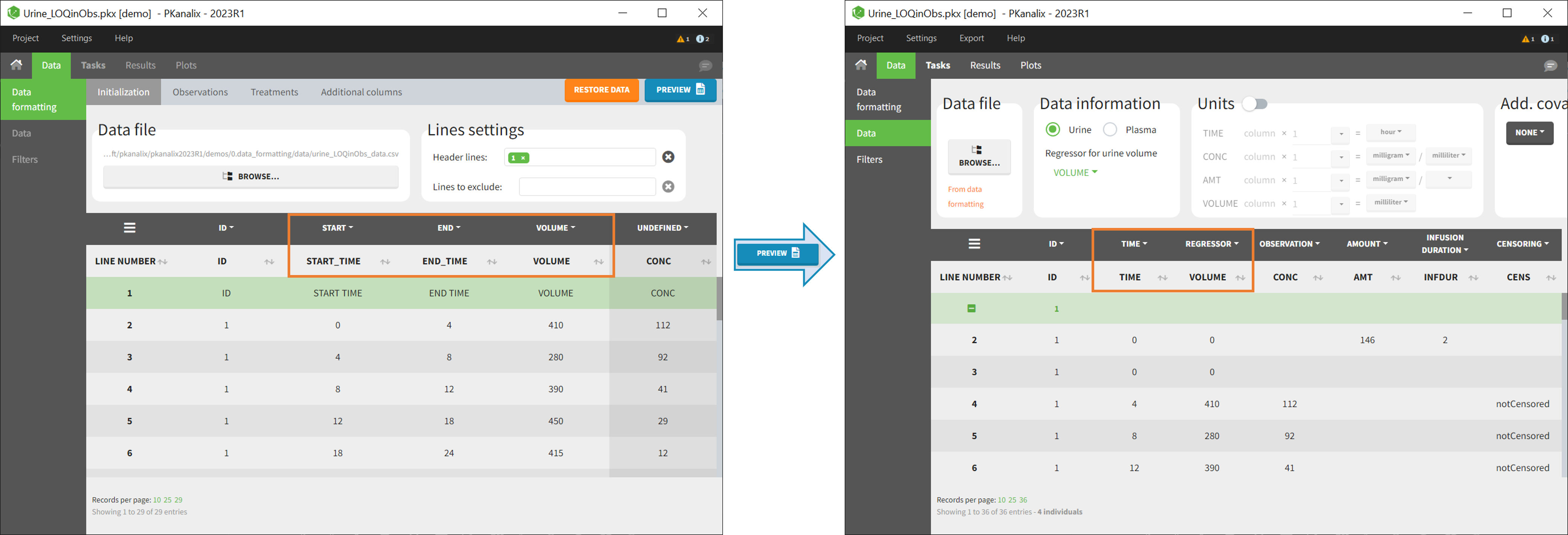
In PKanalix-standard format, the start and end times of urine collection intervals must be recorded in a single column, tagged as TIME column-type, where the end time of an interval automatically acts as start time for the next interval (see here for more details). If a dataset contains start and end times in two different columns, they can be merged into a single column by Data Formatting. This is done automatically by tagging these two columns as START and END in the Initialization subtab of Data Formatting (see Section 2). In addition the column containing urine collection volume must be tagged as VOLUME.
Example:
- demo Urine_LOQinObs.plx:
11. Adding new columns from an external file
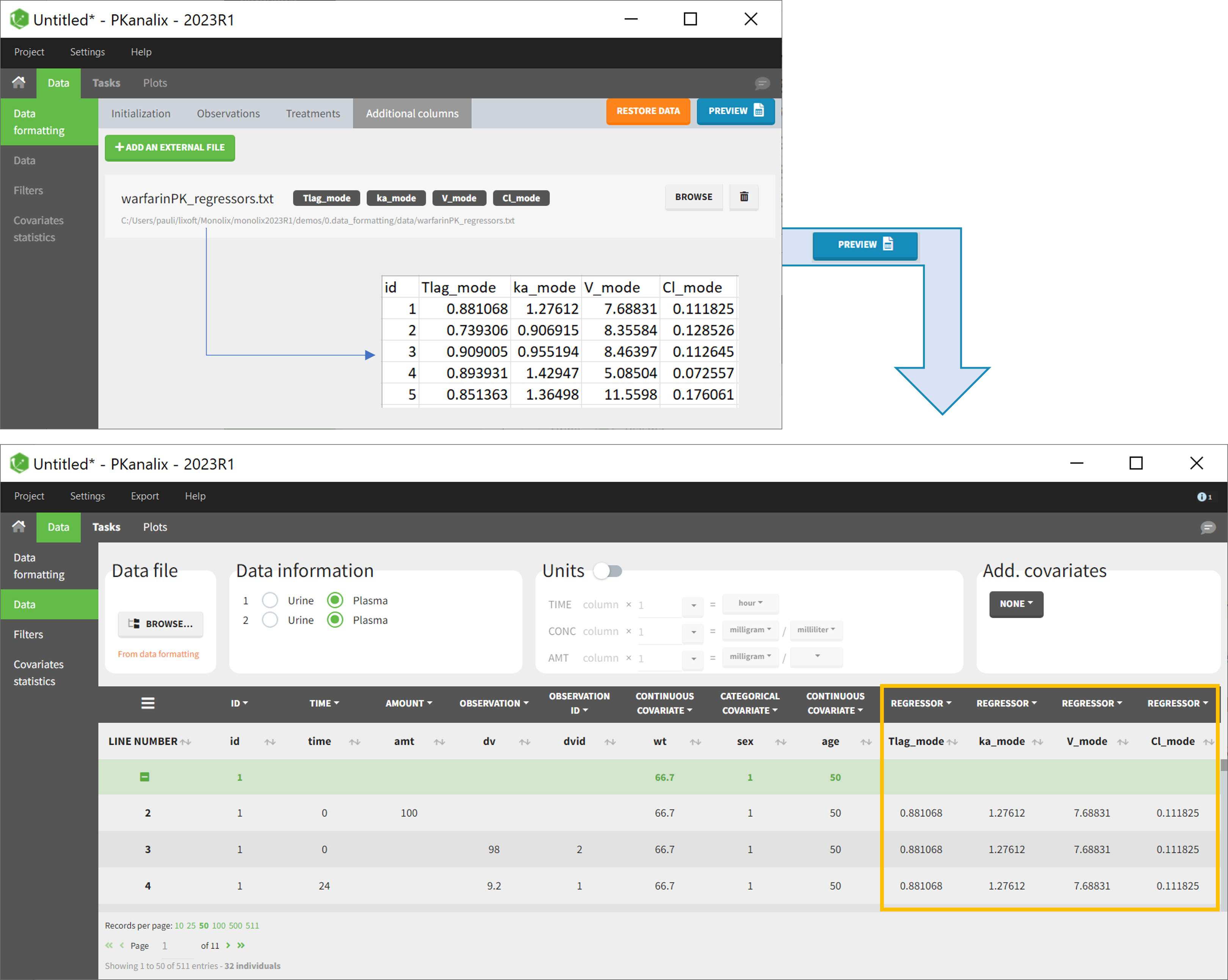
The last subtab is used to insert additional columns in the dataset from a separate file. The external file must contain a table with a column named ID or id with the same subject identifiers as in the dataset to format, and other columns with a header name and individual values (numbers or strings). There can be only one value per individual, which means that the additional columns inserted in the formatted dataset can contain only a constant value within each individual, and not time-varying values.
Examples of additional columns that can be added with this option are:
- individual parameters estimated in a previous analysis, to be read as regressors to avoid estimating them. Time-varying regressors are not handled.
- new covariates.
If occasions are defined in the formatted dataset, it is possible to have an occasion column in the external file and values defined per subject-occasion.
Example:
- demo warfarin_PKPDseq_project.mlxtran (Monolix demo in the folder 0.data_formatting, here imported into PKanalix):
This demo imported from a Monolix demo has an initial PKPD dataset in Monolix-standard format. The option “Additional columns” is used to add the PK parameters estimated on the PK part of the data in another Monolix project.
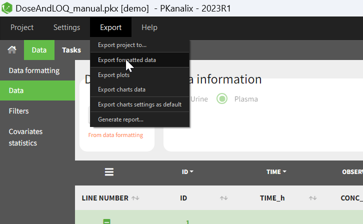
12. Exporting the formatted dataset
Once data formatting is done and the new dataset is accepted, the project can be saved and it is possible to export the formatted dataset as a csv file from the main menu Export > Export formatted data.