
1.PKanalix documentation
Version 2024
This documentation is for PKanalix.
©Lixoft
PKanalix performs analysis on PK data set including:
- The non compartmental analysis (NCA) – computation of the NCA parameters using the calculation of the \(\lambda_z\) – slope of the terminal elimination phase.
- The bioequivalence analysis (BE) – comparison of the NCA parameters of several drug products (usually two, called ‘test’ and ‘reference’) using the average bioequivalence.
- The compartmental analysis (CA) – estimation of model parameters representing the PK as the dynamics in compartments for each individual. It does not include population analysis performed in Monolix.
What else?
- A clear user-interface with an intuitive workflow to efficiently run the NCA, BE and CA analysis.
- Easily accessible PK models library and auto-initialization method to improve the convergence of the optimization of CA parameters.
- Integrated bioequivalence module to simplify the analysis
- Automatically generated results and plots to give an immediate feedback.
- Interconnection with MonolixSuite applications to export projects to Monolix for the population analysis.
PKanalix tasks
Pkanalix uses the dataset format common for all MonolixSuite applications, see here for more details. It allows to move your project between applications, for instance export a CA project to Monolix and perform a population analysis with one “click” of a button.
Non Compartmental Analysis |
Bioequivalence |
Compartmental Analysis |
| This task consists in defining rules for the calculation of the \(\lambda_z\) (slope of the terminal elimination phase) to compute all the NCA parameters. This definition can be either global via general rules or manual on each individual – with the interactive plots the user selects or removes points in the \(\lambda_z\) calculation. |
The average NCA parameters obtained for different groups (e.g a test and a reference formulation) can be compared using the Bioequivalence task. Linear model definition contains one or several fixed effects selected in an integrated module. It allows to obtain a confidence interval compared to the predefined BE limits and automatically displayed in intuitive tables and plots. |
This task estimates parameters of a pharmacokinetic model for each individual. The model can be custom or based on one of the user-friendly libraries. Automatic initialization method improves the convergence of parameters for each individual. |
All the NCA, BE and/or CA outputs are automatically displayed in sortable tables in the Results tab. Moreover, they are exported in the result folder in a R-compatible format. Interactive plots give an immediate feedback and help to better interpret the results.
The usage of PKanalix is available not only via the user interface, but also via R with a dedicated R-package (detailed here). All the actions performed in the interface have their equivalent R-functions. It is particularly convenient for reproducibility purpose or batch jobs.
The results of the NCA calculations and bioequivalence calculations have been compared on an extensive number of datasets to the results of WinNonLin and to published results obtained with SAS. All results were identical. See the poster below for more details.
2.Data
2.1.Defining a dataset
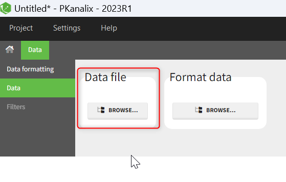
To start a new PKanalix project, you need to define a dataset by loading a file in the Data tab.
Supported file types: Supported file types include .txt, .csv, and .tsv files. Starting with version 2024, additional Excel and SAS file types are supported: .xls, .xlsx, .sas2bdat, and .xpt files in addition to .txt, .csv, and .tsv files.
The data set format expected in the Data tab is the same as for the entire MonolixSuite, to allow smooth transitions between applications. The columns available in this format and example datasets are detailed on this page. Briefly:
- Each line corresponds to one individual and one time point
- Each line can include a single measurement (also called observation), or a dose amount (or both a measurement and a dose amount)
- Dosing information should be indicated for each individual, even if it is identical for all.
Your dataset may not be originally in this format, and you may want to add information on dose amounts, limits of quantification, units, or filter part of the dataset. To do so, you should proceed in this order:
- 1) Formatting: If needed, format your data first by loading the dataset in the Data Formatting tab. Briefly, it allows to:
- to deal with several header lines
- merge several observation columns into one
- add censoring information based on tags in the observation column
- add treatment information manually or from external sources
- add more columns based on another file
or
- 1) If the data is already in the right format, load it directly in the Data tab (otherwise use the formatted dataset created by data formatting). If the dataset does not follow a formatting rule, the dataset will not be accepted, but errors will guide you to find what is missing and could be added by data formatting.
- 2) Labeling: label the columns not recognized automatically to indicate their type and click on ACCEPT.
- 3) Units: If you want to work with units, indicate the units in the data and the ones you prefer to use inside the Data tab (if relevant)
- 4) Filters: If needed, filter your dataset to use only part of it in the Filters tab
- 5) Explore: The interpreted dataset is displayed in Data, and Plots and covariate statistics are generated.
To use a dataset from a Monolix project, or to use simulations from a Simulx project, you can directly import or export the Monolix/Simulx project which will automatically define the dataset in the data tab.
Labeling
The column type suggested automatically by PKanalix based on the headers in the data can be customized in the preferences. By clicking on Settings>Preferences, the following windows pops up.

In the DATA frame, you can add or remove preferences for each column.
To remove a preference, double-click on the preference you would like to remove. A confirmation window will be proposed.
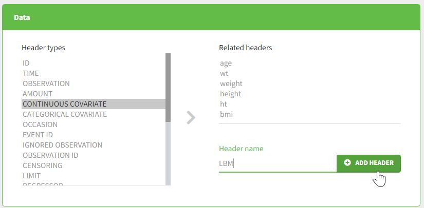
To add a preference, click on the header type you consider, add a name in the header name and click on “ADD HEADER” as on the following figure.
Notice that all the preferences are shared between Monolix, Datxplore, and PKanalix.
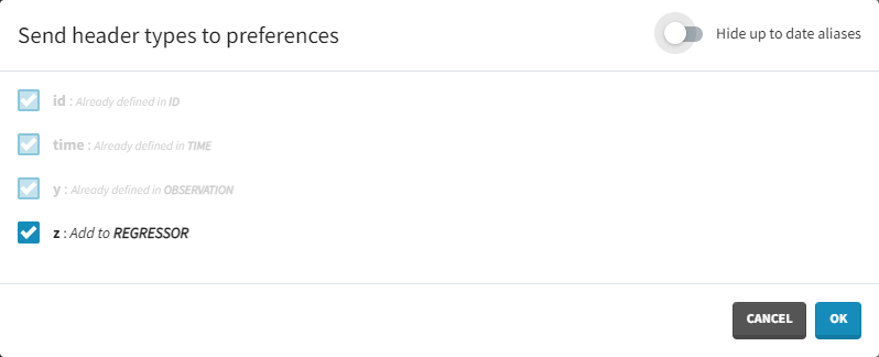
Starting from the version 2024, it is also possible to update the preferences with the columns tagged in the opened project, by clicking on the icon in the top left corner of the table:
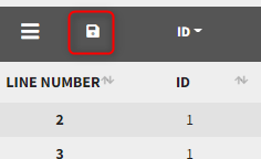
Clicking on the icon will open a modal with the option to choose which of the tagged headers a user wants to add to preferences:
Dataset load times
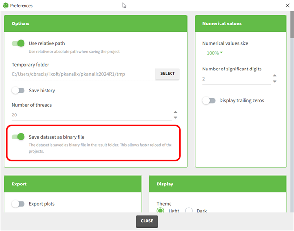
Starting with the 2024 version, it is possible to improve the project load times, especially for projects with large datasets, but saving the data as a binary file. This option is available in Settings>Preferences and will save a copy of the data file in binary format in the results folder. When reloading a project, the dataset will be read from the binary file, which will be faster. If the original dataset file has been modified (compared to the binary), a warning message will appear, the binary dataset will not be used and the original dataset fiel will be loaded instead.
Resulting plots and tables to explore the data
Once the dataset is accepted:
- Plots are automatically generated based on the interpreted dataset to help you proceed with a first data exploration before running any task.
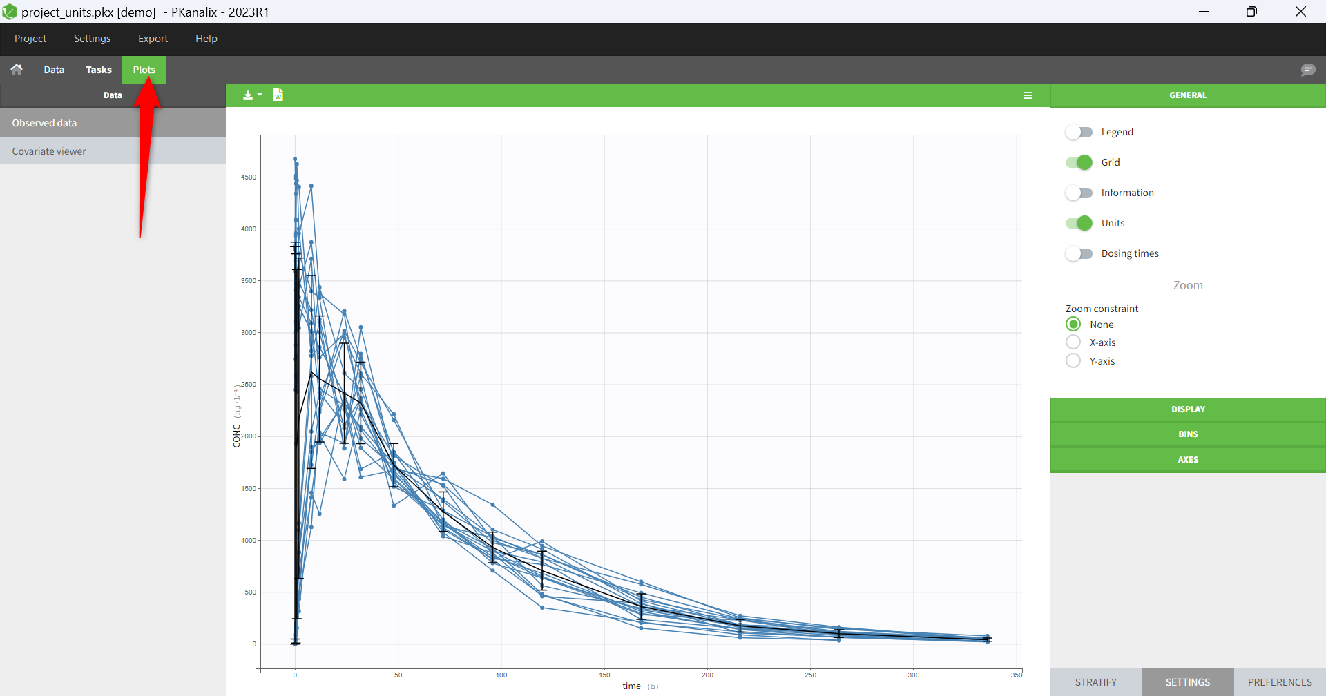
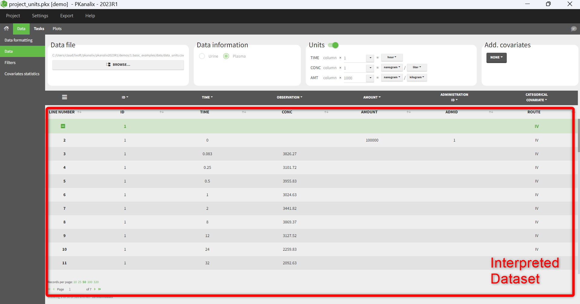
- The interpreted dataset appears in Data tab, which incorporates all changes after formatting, setting units, and filtering.
- Covariate Statistics appear in a section of the data tab.
2.2.Data format for NCA and CA analysis
In PKanalix, a dataset should be loaded in the Data tab to create a project. Once the dataset accepted, it is possible to specify units and filter the dataset, so units and filtering information should not be included in the file loaded in the Data tab.
The data set format used in PKanalix is the same as for the entire MonolixSuite, to allow smooth transitions between applications. In this format:
- Each line corresponds to one individual and one time point.
- Each line can include a single measurement (also called observation), or a dose amount (or both a measurement and a dose amount).
- Dosing information should be indicated for each individual in a specific column, even if it is the same treatment for all individuals.
- Headers are free but there can be only one header line.
- Different types of information (dose, observation, covariate, etc) are recorded in different columns, which must be tagged with a column type (see below).
If your dataset is not in this format, in most cases, it is possible to format it in a few steps in the data formatting tab, to incorporate the missing information.
- Overview of most common column types
- Example datasets
- Plasma concentration data
- Steady-state data
- BLQ data
- Urine data
- Occasions (“Sort” variables)
- Covariates (“Carry” variables)
- Other useful column-types
- Description of all possible column types
Overview of most common column-types
A data set typically contains only the following columns: ID (mandatory), TIME (mandatory), OBSERVATION (mandatiry), AMOUNT (optional). The main rules for interpreting the dataset are:
- Cells that do not contain information (e.g AMOUNT column on a line recording a measurement) should have a dot.
- Headers are free but there can be only one header line and the columns must be assigned to one of the available column-types. The full list of column-types is available at the end of this page and a detailed description is given on the dataset documentation website.
The most common column types in addition to ID, TIME, OBSERVATION and AMOUNT are:
- For IV infusion data, an additional INFUSION RATE or INFUSION DURATION is necessary.
- For steady-state data, either an INTERDOSE INTERVAL column is added, or the interdose interval tau is specified in the NCA settings.
- If a dose and a measurement occur at the same time, they can be encoded on the same line or on different lines.
- Sort and carry variables can be defined using the OCCASION, and CATEGORICAL COVARIATE and CONTINUOUS COVARIATE column-types.
- BLQ data are defined using the CENSORING and LIMIT column-types.
In addition to the typical cases presented above, a few additional column-types may also be convenient:
- ignoring a line: with the IGNORED OBSERVATION (ignores the measurement only) or IGNORED LINE (ignores the entire line, including regressor and dose information). However it is more convenient to filter lines of your dataset without modifying it by using filters (available once your dataset is accepted).
- working with several types of observations: If several observation types are present in the dataset (for example parent and metabolite), all measurements should still appear in the same OBSERVATION column, and another column should be used to distinguish the observation types. If this is not the case in your dataset, data formatting enables to merge several observation columns. To run NCA for several observations at the same time for the same id, tag the column listing the observation types as OCCASION . To run CA for several observations with a model including several outputs (for example PK and PD), tag the column listing the observation types as OBSERVATION ID. In this case, only one observation type will be available for NCA. It can be selected in the “NCA” section to perform the calculations.
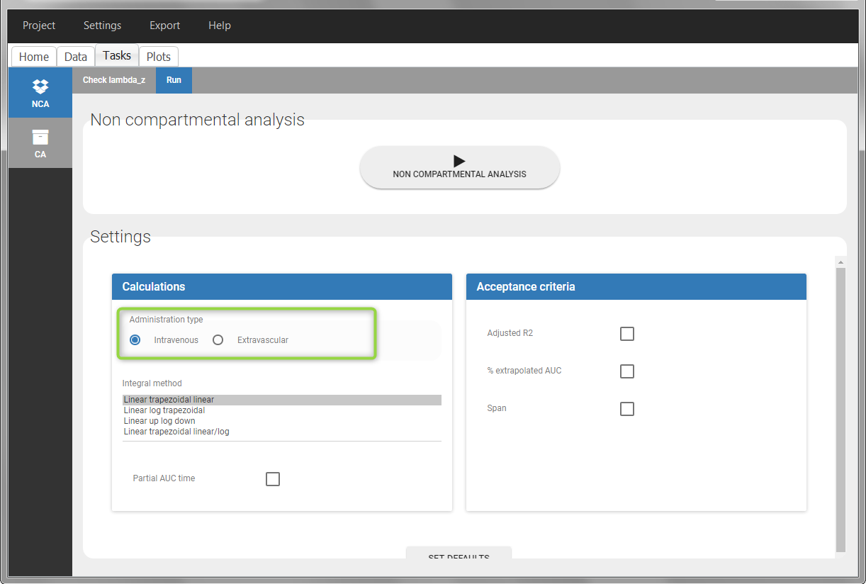
- working with several types of administrations: a single data set can contain different types of administrations, for instance IV bolus and extravascular, distinguished using the ADMINISTRATION ID column-type. The setting “administration type” in “Tasks>Run” can be chosen separately for each administration id, and the appropriate parameter calculations will be performed.
Example datasets
Below we show how to encode the dataset for most typical situations.
Plasma concentration data
Extravascular
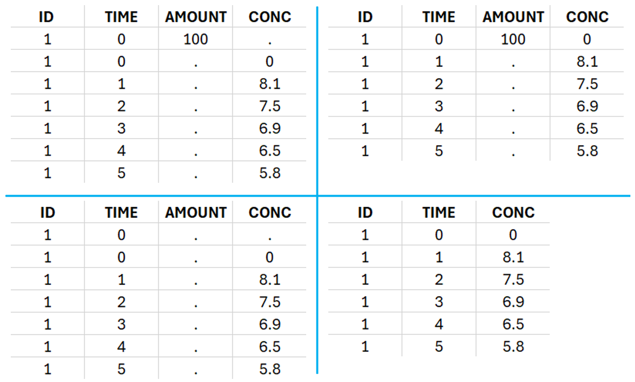
For extravascular administration, the mandatory column-types are ID (individual identifiers as integers or strings), OBSERVATION (measured concentrations), AMOUNT (dose amount administered, mandatory for 2023 and previous versions) and TIME (time of dose or measurement). Since version 2024, datasets that do not contain an AMOUNT column or no information in the AMOUT column are accepted for single dose or multiple dose administrations.
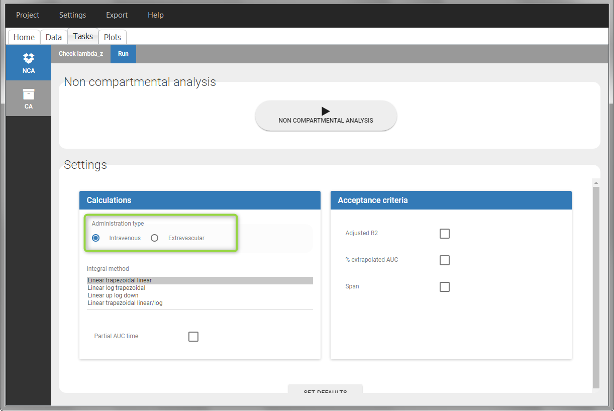
To distinguish the extravascular from the IV bolus case, in “Tasks>Run” the administration type must be set to “extravascular”.
If no measurement is recorded at the time of the dose, a concentration of zero is added for single dose data, the minimum concentration observed during the dose interval for steady-state data.
Example:
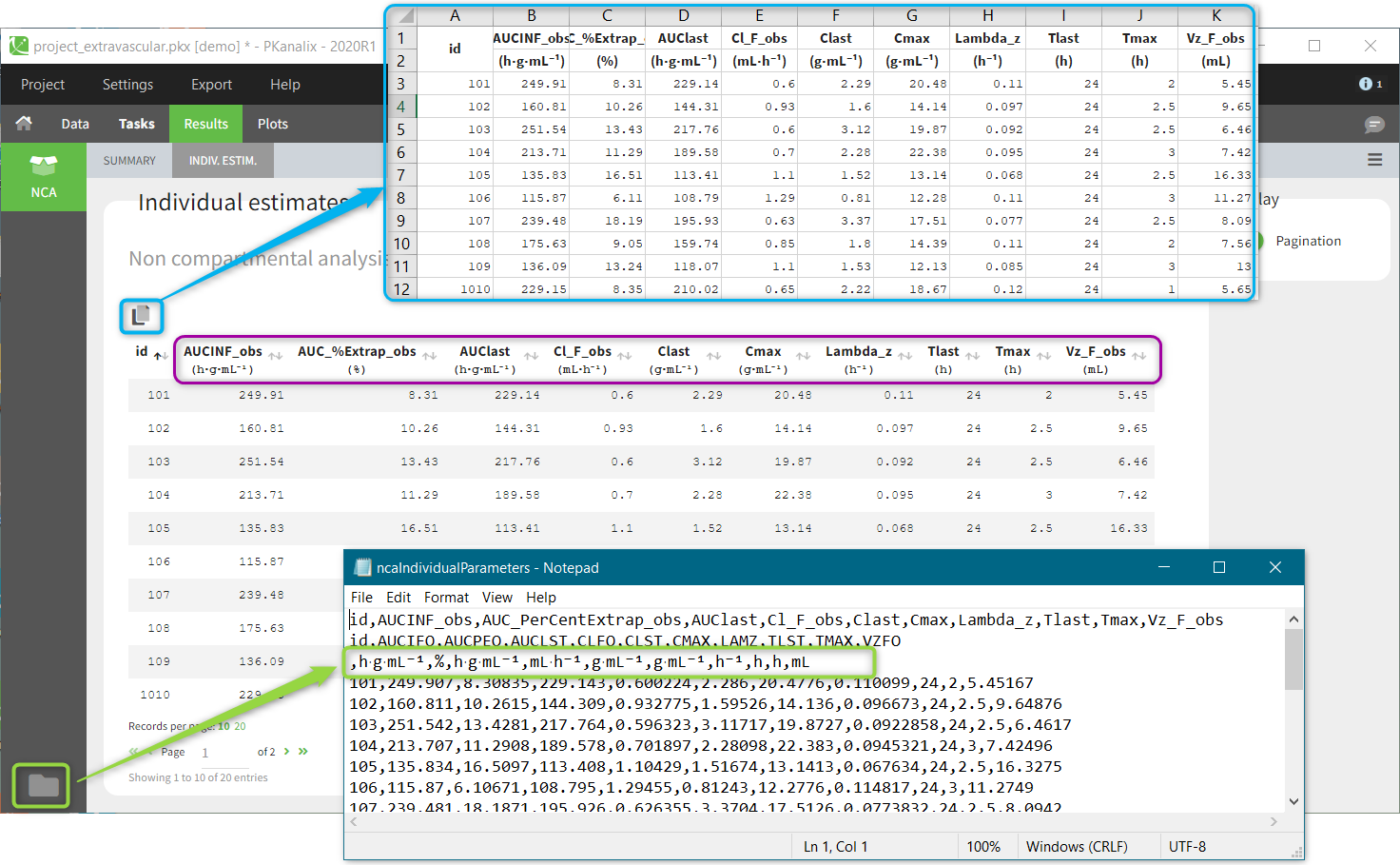
- demo project_extravascular.pkx
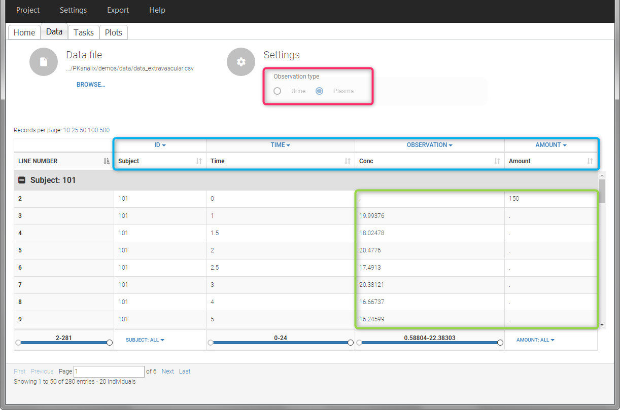
This data set records the drug concentration measured after single oral administration of 150 mg of drug in 20 patients. For each individual, the first line records the dose (in the “Amount” column tagged as AMOUNT column-type) while the following lines record the measured concentrations (in the “Conc” column tagged as OBSERVATION). Cells of the “Amount” column on measurement lines contain a dot, and respectively for the concentration column. The column containing the times of measurements or doses is tagged as TIME column-type and the subject identifiers, which we will use as sort variable, are tagged as ID. Check the OCCASION section if more sort variables are needed. After accepting the dataset, the data is automatically assigned as “Plasma”.
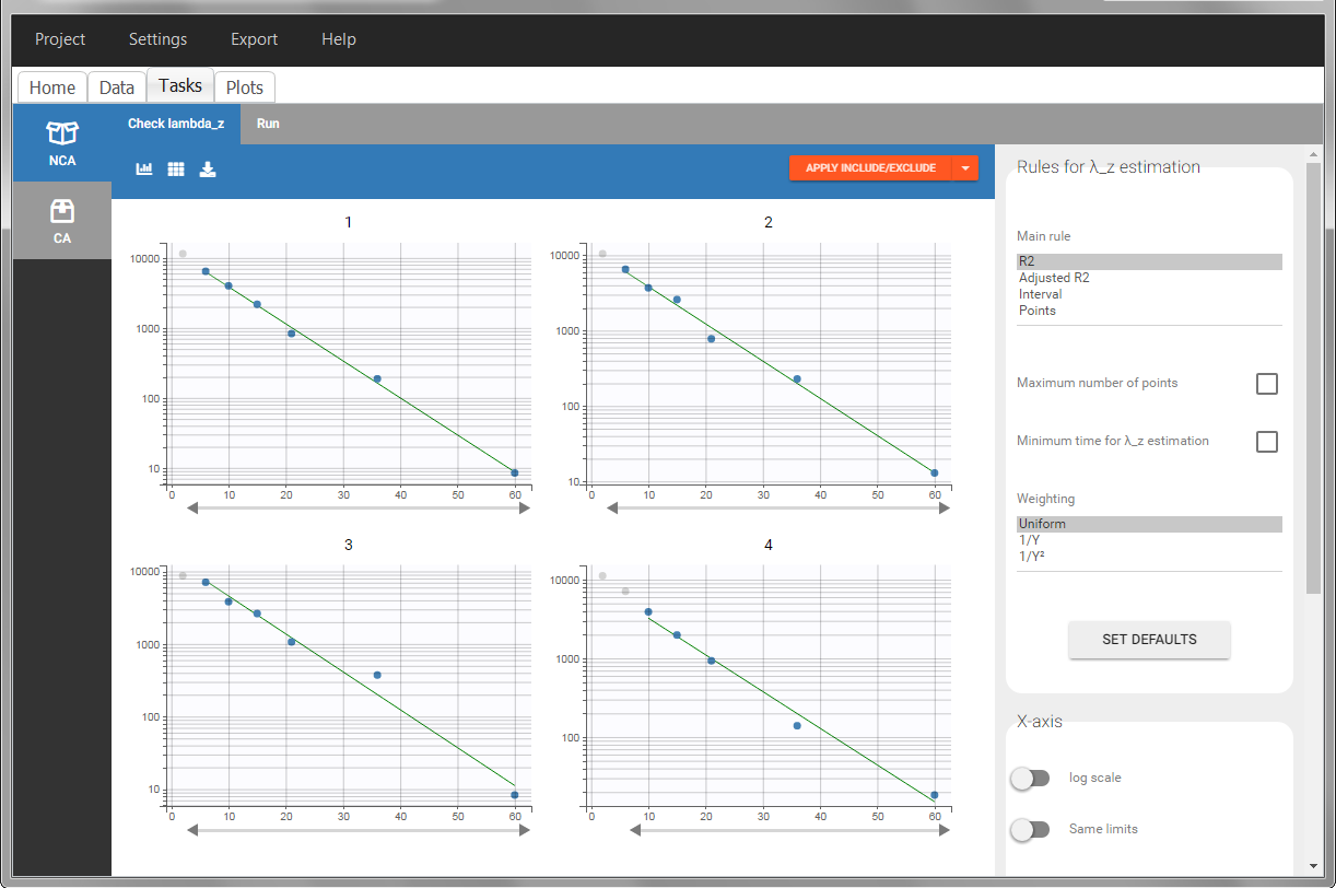
In the “Tasks/Run” tab, the user must indicate that this is extravascular data. In the “Check lambda_z”, on linear scale for the y-axis, measurements originally present in the data are shown with full circles. Added data points, such as a zero concentration at the dose time, are represented with empty circles. Points included in the \(\lambda_z\) calculation are highlighted in blue.
 |
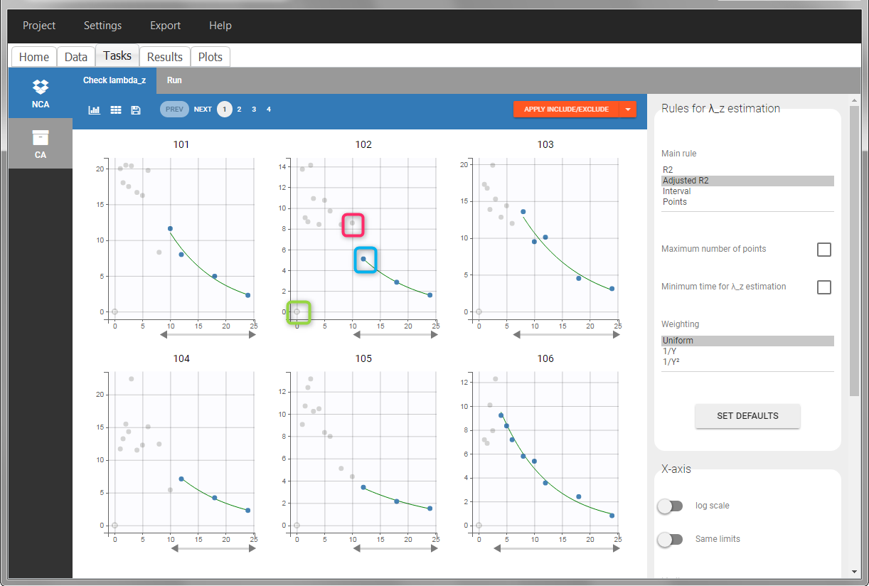 |
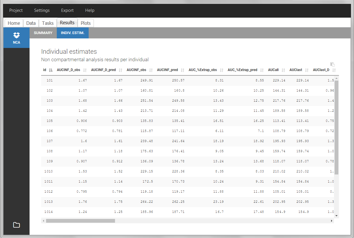
After running the NCA analysis, PK parameters relevant to extravascular administration are displayed in the “Results” tab.
IV infusion
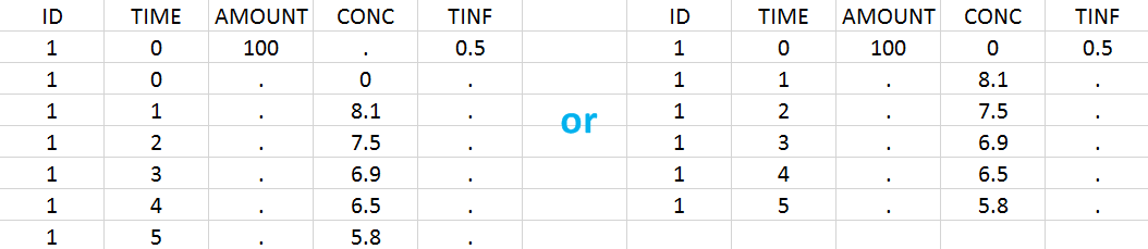
Intravenous infusions are indicated in the data set via the presence of an INFUSION RATE or INFUSION DURATION column-type, in addition to the ID (individual identifiers as integers or strings), OBSERVATION (measured concentrations), AMOUNT (dose amount administered, mandatory for 2023 and previous versions) and TIME (time of dose or measurement). The infusion duration (or rate) can be identical or different between individuals. Since version 2024, datasets that do not contain an AMOUNT column or no information in the AMOUT column are accepted for single dose or multiple dose administrations.
In “Tasks>Run” the administration type must be set to “intravenous”.
If no measurement is recorded at the time of the dose, a concentration of zero is added for single dose data, the minimum concentration observed during the dose interval for steady-state data.
Example:
- demo project_ivinfusion.pkx:
In this example, the patients receive an iv infusion over 3 hours. The infusion duration is recorded in the column called “TINF” in this example, and tagged as INFUSION DURATION.
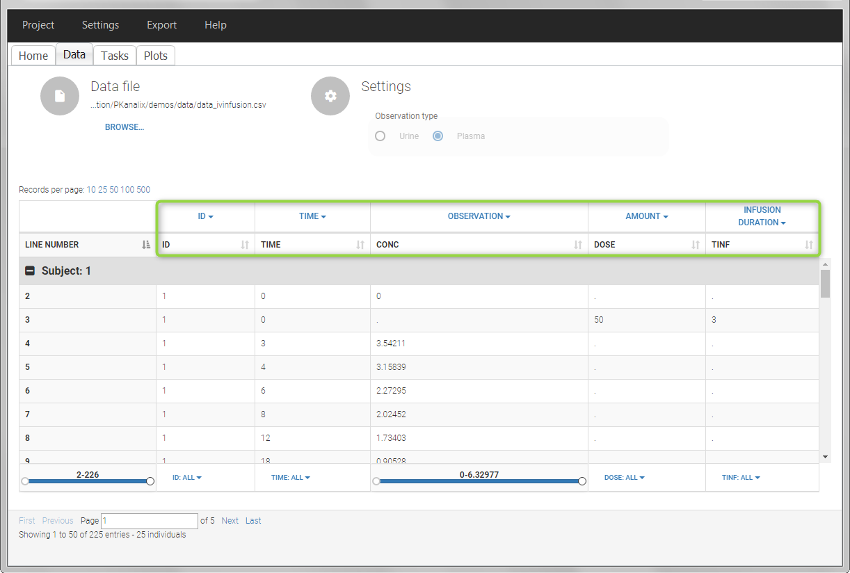
In the “Tasks/Run” tab, the user must indicate that this is intravenous data.
IV bolus
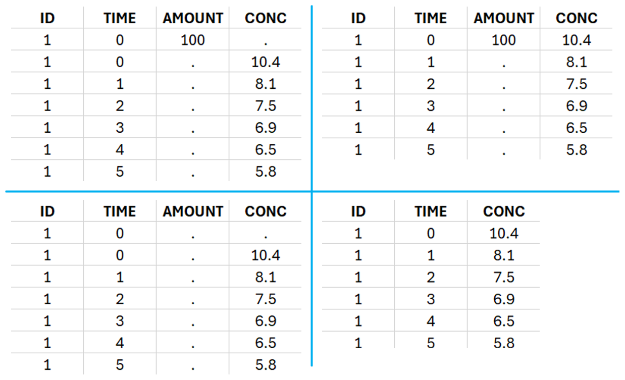
For IV bolus administration, the mandatory column-types are ID (individual identifiers as integers or strings), OBSERVATION (measured concentrations), AMOUNT (dose amount administered, mandatory for 2023 and previous versions) and TIME (time of dose or measurement). Since version 2024, datasets that do not contain an AMOUNT column or no information in the AMOUT column are accepted for single dose or multiple dose administrations.
To distinguish the IV bolus from the extravascular case, in “Tasks>Run” the administration type must be set to “intravenous”.
If no measurement is recorded at the time of the dose, the concentration of at time zero is extrapolated using a log-linear regression of the first two data points, or is taken to be the first observed measurement if the regression yields a slope >= 0. See the calculation details for more information.
Example:
- demo project_ivbolus.pkx:
In this data set, 25 individuals have received an iv bolus and their plasma concentration have been recorded over 12 hours. For each individual (indicated in the column “Subj” tagged as ID column-type), we record the dose amount in a column “Dose”, tagged as AMOUNT column-type. The measured concentrations are tagged as OBSERVATION and the times as TIME. Check the OCCASION section if more sort variables are needed in addition to ID. After accepting the dataset, the data is automatically assigned as “plasma”.
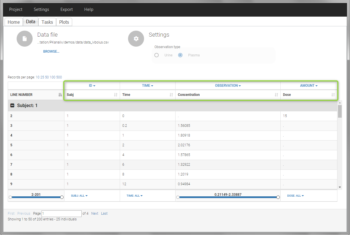
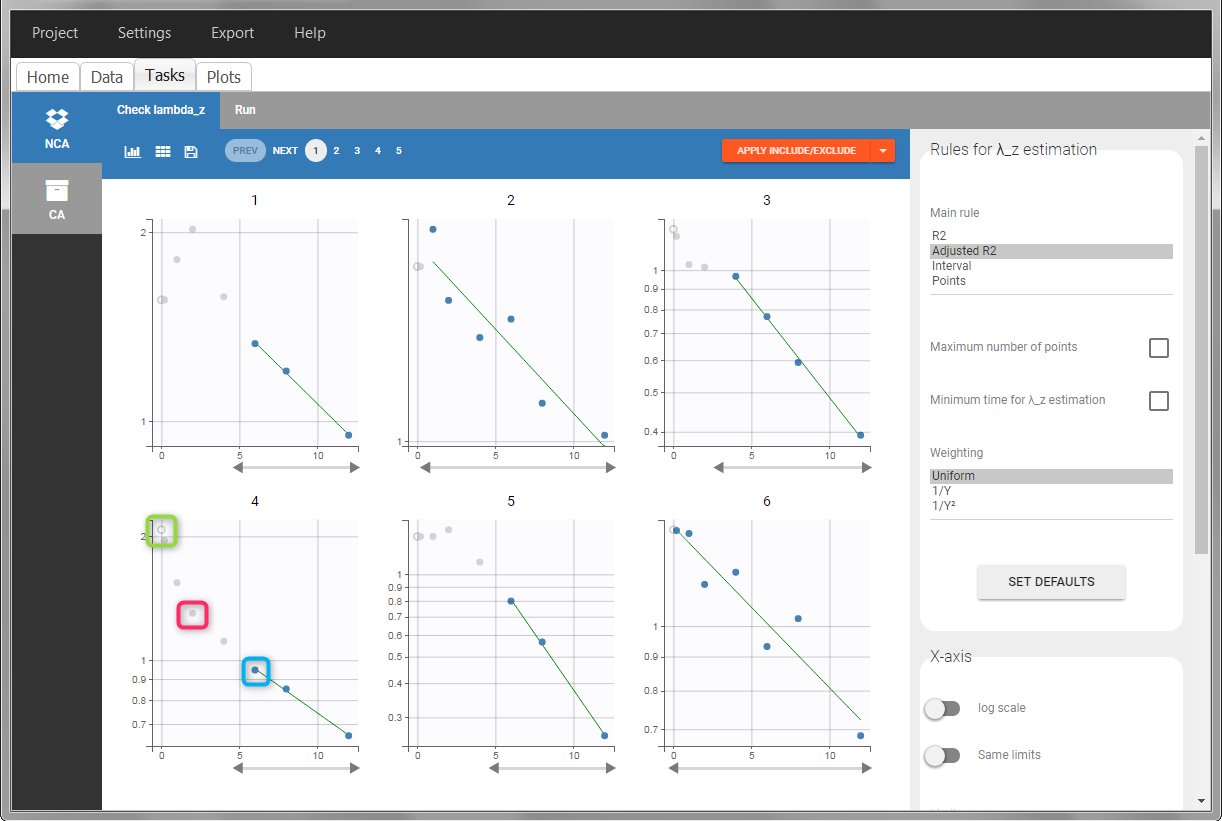
In the “Tasks/Run” tab, the user must indicate that this is intravenous data. In the “Check lambda_z”, measurements originally present in the data are shown with full circles. Added data points, such as the C0 at the dose time, are represented with empty circles. Points included in the \(\lambda_z\) calculation are highlighted in blue.
 |
 |
After running the NCA analysis, PK parameters relevant to iv bolus administration are displayed in the “Results” tab.
Steady-state
Starting from version 2024, the interdose interval tau used to calculate NCA parameters specific to steady-state can be specified either in the dataset column tagged as INTERDOSE INTERVAL, or directly as part of the NCA settings.
In the 2023 and previous versions, it was necessary to indicate steady-state using the STEADY STATE column-type: SS=1 indicates that the individual is already at steady-state when receiving the dose. This implicitly assumes that the individual has received many doses before this one. SS=0 or ‘.’ indicates a single dose. Starting from version 2024, the SS column is accepted but not mandatory anymore.
The dosing interval (also called tau) is indicated in the INTERDOSE INTERVAL column on the lines defining the doses, or as part of the NCA settings.
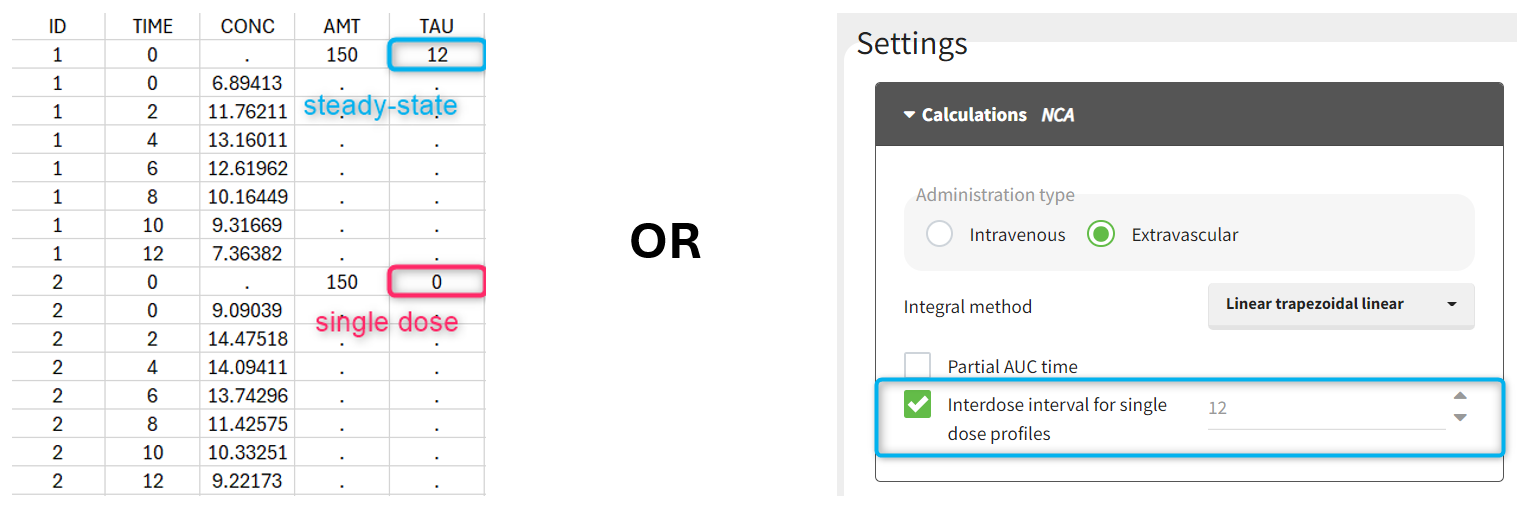
Steady state calculation formulas will be applied for individuals having a dose with INTERDOSE INTERVAL = double. A data set can contain individuals which are at steady-state and some which are not. If the NCA setting “Interdose interval for single dose profiles” is selected, steady-state parameters are calculated for all individuals.
If no measurement is recorded at the time of the dose, the minimum concentration observed during the dose interval is added at the time of the dose for extravascular and infusion data. For iv bolus, a regression using the two first data points is performed. Only measurements between the dose time and dose time + interdose interval will be used.
Examples:
- demo project_steadystate.pkx:
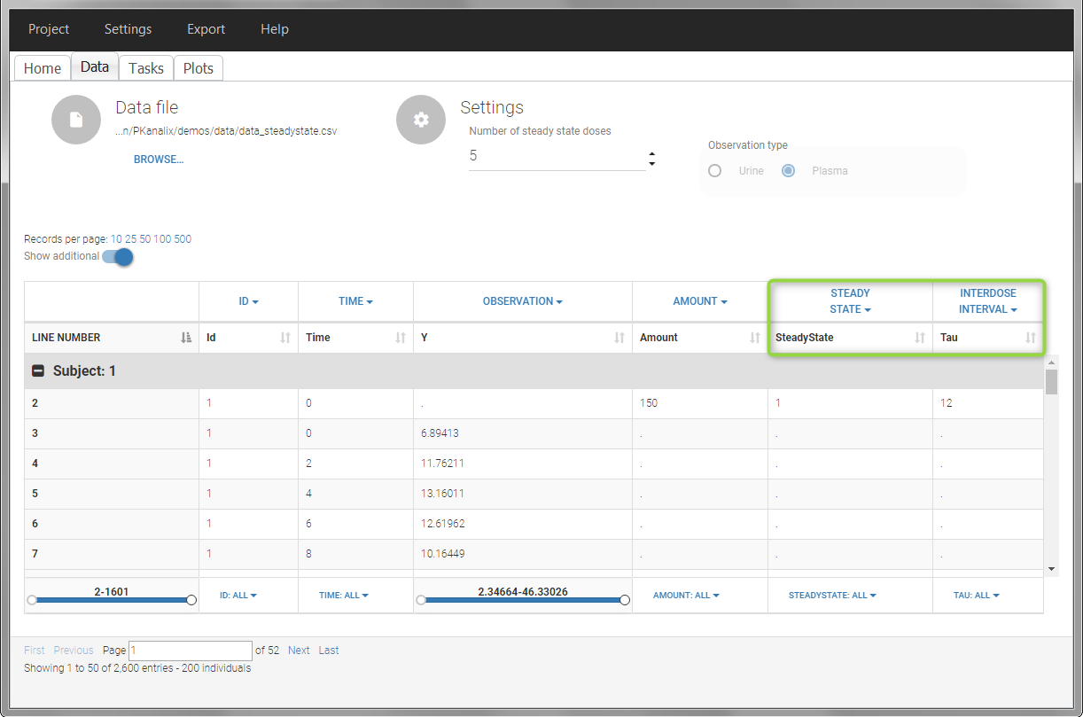
In this example, the individuals are already at steady-state when they receive the dose. This is indicated in the data set via the column “SteadyState” tagged as STEADY STATE column-type, which contains a “1” on lines recording doses. The interdose interval is noted on those same line in the column “tau” tagged as INTERDOSE INTERVAL. When accepting the data set, a “Settings” section appears, which allows to define the number of steady-state doses. This information is relevant when exporting to Monolix, but not used in PKanalix directly.
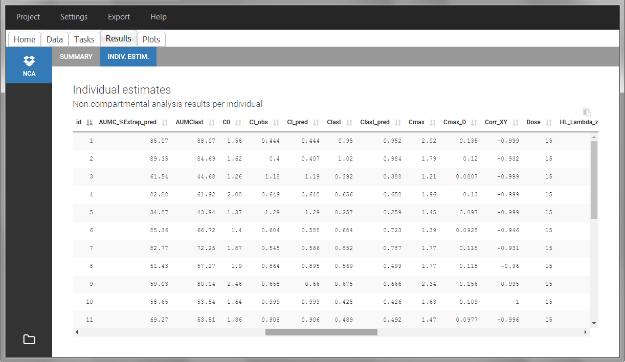
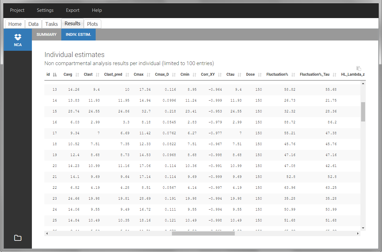
After running the NCA estimation task, steady-state specific parameters are displayed in the “Results” tab.
BLQ data
Below the limit of quantification (BLQ) data can be recorded in the data set using the CENSORING column:
- “0” indicates that the value in the OBSERVATION column is the measurement.
- “1” indicates that the observation is BLQ.
The lower limit of quantification (LOQ) must be indicated in the OBSERVATION column when CENSORING = “1”. Note that strings are not allowed in the OBSERVATION column (except dots). A different LOQ value can be used for each BLQ data.
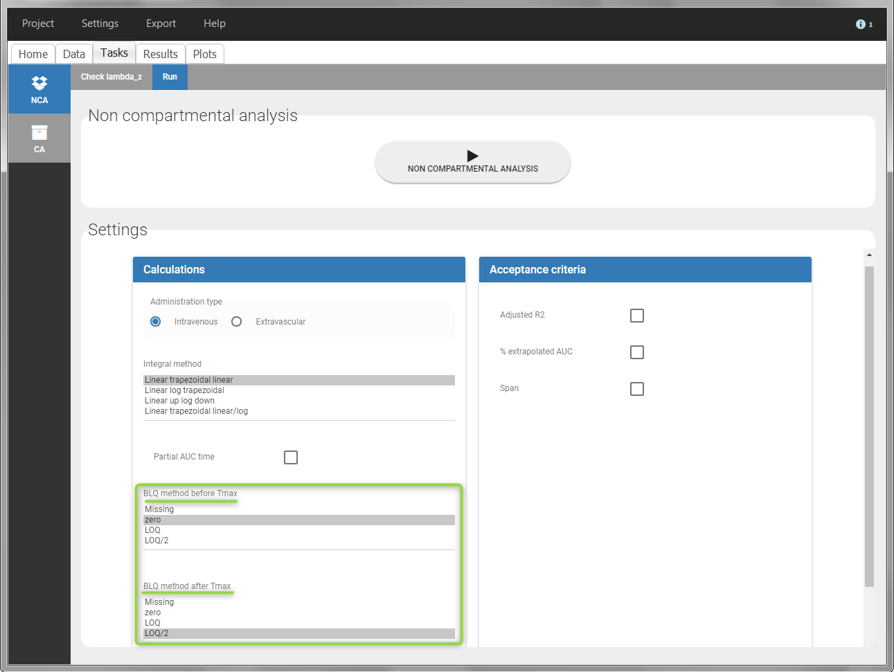
When performing an NCA analysis, the BLQ data before and after the Tmax are distinguished. They can be replaced by:
- zero
- the LOQ value
- the LOQ value divided by 2
- or considered as missing
For a CA analysis, the same options are available, but no distinction is done between before and after Tmax. Once replaced, the BLQ data are handled as any other observation.
A LIMIT column can be added to record the other limit of the interval (in general zero). This value will not be used by PKanalix but can facilitate the transition from an NCA/CA analysis PKanalix to a population model with Monolix.
To easily encode BLQ data in a dataset that only has BLQ tags in the observation column, you can use Data formatting.
Examples:
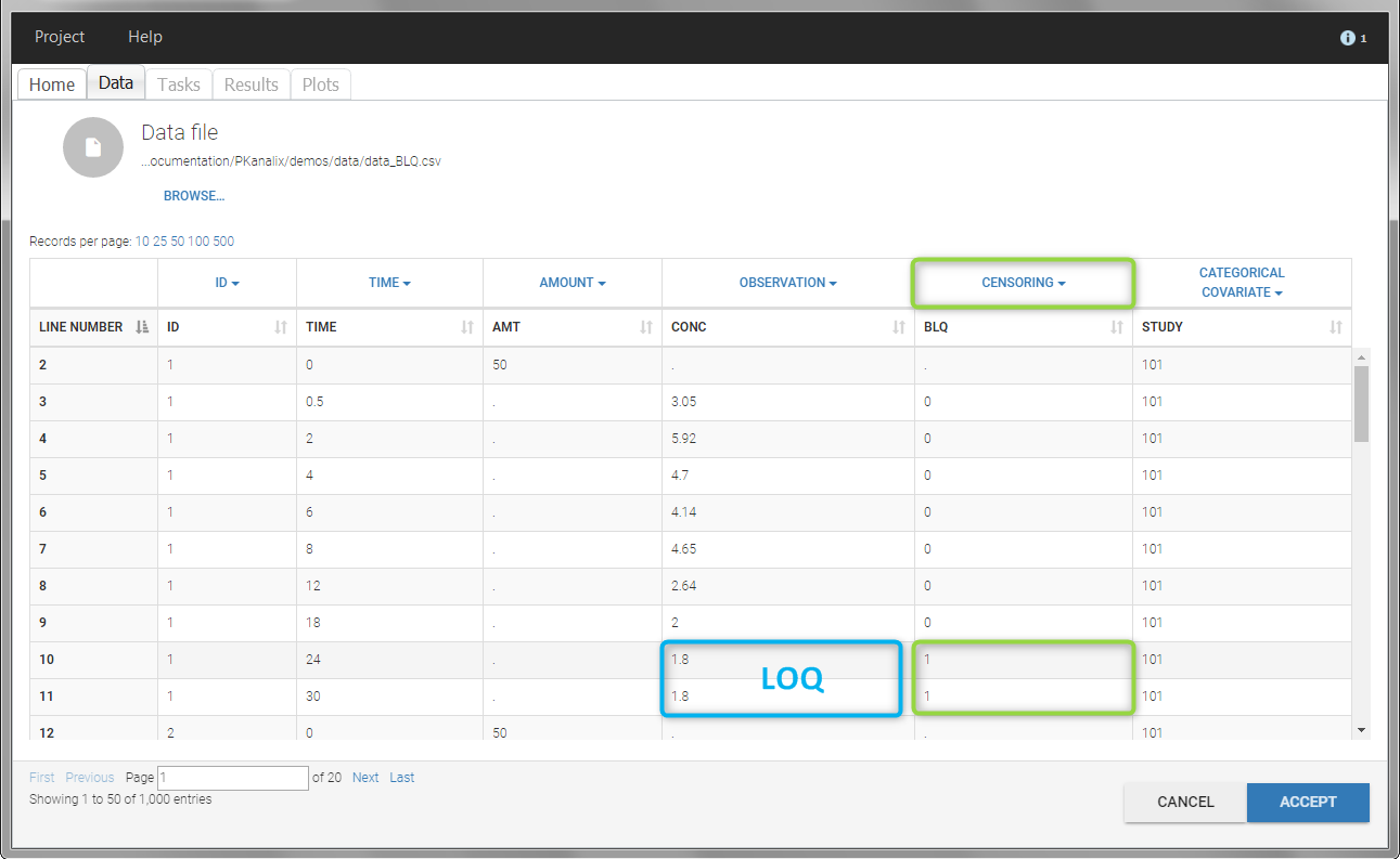
- demo project_censoring.pkx: two studies with BLQ data with two different LOQ
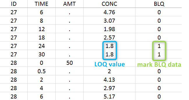
In this dataset, the measurements of two different studies (indicated in the STUDY column, tagged as CATEGORICAL COVARIATE in order to be carried over) are recorded. For the study 101, the LOQ is 1.8 ug/mL, while it is 1 ug/mL for study 102. The BLQ data are marked with a “1” in the BLQ column, which is tagged as CENSORING. The LOQ values are indicated for each BLQ in the CONC column of measurements, tagged as OBSERVATION.
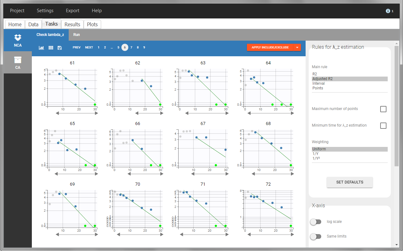
In the “Task>NCA>Run” tab, the user can choose how to handle the BLQ data. For the BLQ data before and after the Tmax, the BLQ data can be considered as missing (as if this data set row would not exist), or replaced by zero (default before Tmax), the LOQ value or the LOQ value divided by 2 (default after Tmax). In the “Check lambda_z” tab, the BLQ data are shown in green and displayed according to the replacement value.
 |
 |
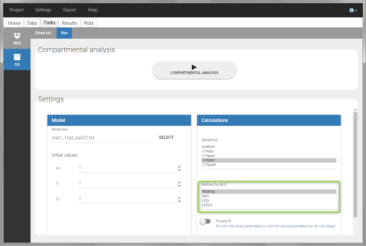
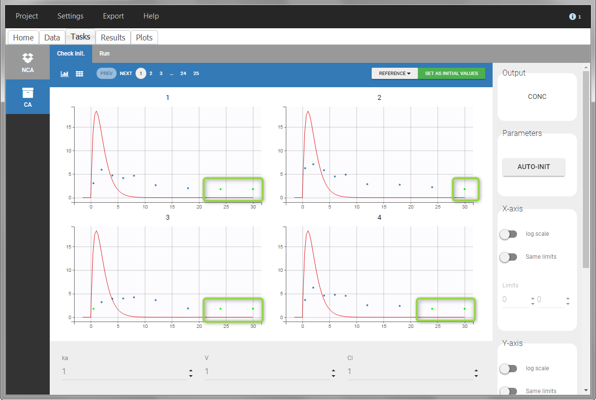
For the CA analysis, the replacement value for all BLQ can be chosen in the settings of the “Run” tab (default is Missing). In the “Check init.” tab, the BLQ are again displayed in green, at the LOQ value (irrespective of the chosen method for the calculations).
 |
 |
Urine data
To work with urine data, it is necessary to record the time and amount administered, the volume of urine collected for each time interval, the start and end time of the intervals and the drug concentration in a urine sample of each interval. The time intervals must be continuous (no gaps allowed).
In PKanalix, the start and end times of the intervals are recorded in a single column, tagged as TIME column-type. In this way, the end time of an interval automatically acts as start time for the next interval. The concentrations are recorded in the OBSERVATION column. The volume column must be tagged as REGRESSOR column type. This general column-type of MonolixSuite data sets allows to easily transition to the other applications of the Suite. As several REGRESSOR columns are allowed, the user can select which REGRESSOR column should be used as volume. The concentration and volume measured for the interval [t1,t2] are noted on the t2 line. The volume value on the dose line is meaningless, but it cannot be a dot. We thus recommend to set it to zero.
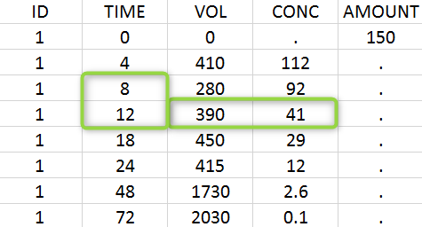
A typical urine data set has the following structure. A dose of 150 ng has been administered at time 0. The first sampling interval spans from the dose at time 0 to 4h post-dose. During this time, 410 mL of urine have been collected. In this sample, the drug concentration is 112 ng/mL. The second interval spans from 4h to 8h, the collected urine volume is 280 mL and its concentration is 92 ng/mL. The third interval is marked on the figure: 390mL of uring have been collected from 8h to 12h.
The given data is used to calculate the intervals midpoints, and the excretion rates for each interval. This information is then used to calculate the \(\lambda_z\) and calculate urine-specific parameters. In “Tasks/Check lambda_z”, we display the midpoints and excretion rates. However, in the “Plots>Data viewer”, we display the measured concentrations at the end time of the interval.
Example:
- demo project_urine.pkx: urine PK dataset
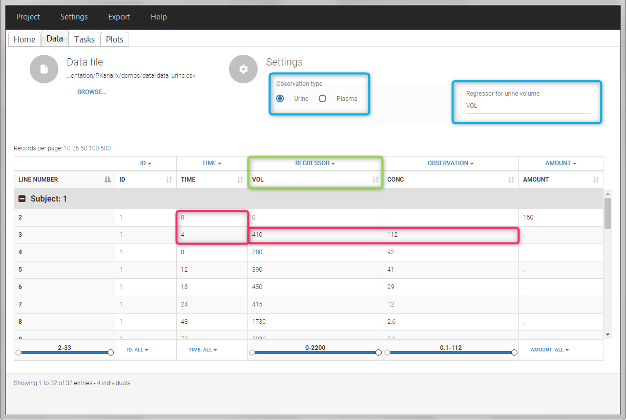
In this urine PK data set, we record the consecutive time intervals in the “TIME” column tagged as TIME. The collected volumes and measured concentration are in the columns “VOL” and “CONC”, respectively tagged as REGRESSOR and OBSERVATION. Note that the volume and concentration are indicated on the line of the interval end time. The volume on the first line (start time of the first interval, as well as dose line) is set to zero as it must be a double. This value will not be used in the calculations. Once the dataset is accepted, the observation type must be set to “urine” and the regressor column corresponding to the volume defined.
In “Tasks>Check lambda_z”, the excretion rate are plotted on the midpoints time for each individual. The choice of the lambda_z works as usual.
Once the NCA task has run, urine-specific PK parameters are displayed in the “Results” tab.

Occasions (“Sort” variables)
The main sort level are the individuals indicated in the ID column. Additional sort levels can be encoded using one or several OCCASION column(s). OCCASION columns contain integer values that permit to distinguish different time periods for a given individual. The time values can restart at zero or continue when switching from one occasion to the next one. The variables differing between periods, such as the treatment for a crossover study, are tagged as CATEGORICAL or CONTINUOUS COVARIATES (see below). The NCA and CA calculations will be performed on each ID-OCCASION combination. Each occasion is considered independent of the other occasions (i.e a washout is applied between each occasion).
Note: occasions columns encoding the sort variables as integers can easily be added to an existing data set using Excel or R.
With R, the “OCC” column can be added to an existing “data” data frame with a column “TREAT” using data$OCC <- ifelse(data$TREAT=="ref", 1, 2).
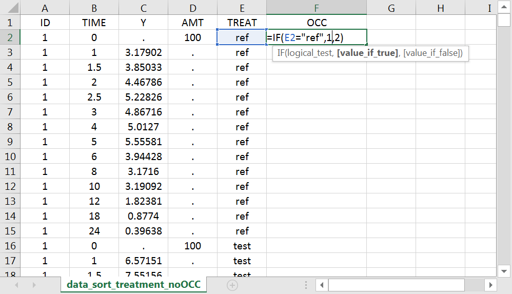
With Excel, assuming the sort variable is encoded in the column E with values “ref” and “test”, type =IF(E2="ref",1,2) to generate the first value of the “OCC” column and then propagate to the entire column:
Examples:
- demo project_occasions1.pkx: crossover study with two treatments
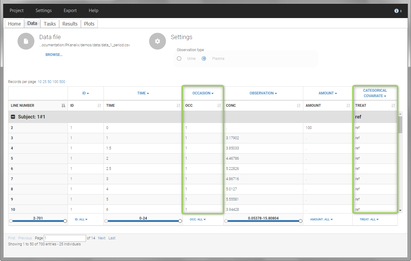
The subject column is tagged as ID, the treatment column as CATEGORICAL COVARIATE and an additional column encoding the two periods with integers “1” and “2” as OCCASION column.
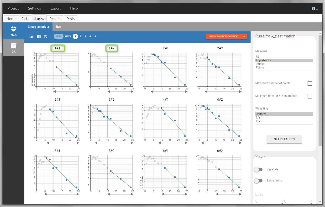
In the “Check lambda_z” (for the NCA) and the “Check init.” (for CA), each occasion of each individual is displayed. The syntax “1#2” indicates individual 1, occasion 2, according to the values defined in the ID and OCCASION columns.
In the “Individual estimates” output tables, the first columns indicate the ID and OCCASION (reusing the data set headers). The covariates are indicated at the end of the table. Note that it is possible to sort the table by any column, including, ID, OCCASION and COVARIATES.
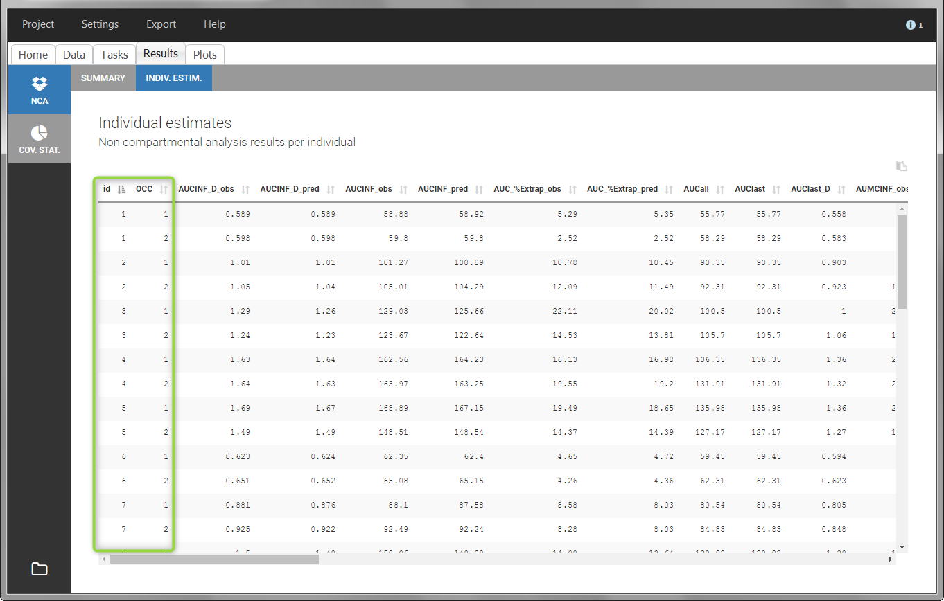
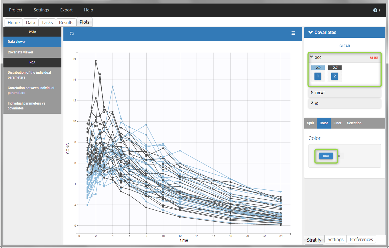
The OCCASION values are available in the plots for stratification, in addition to possible CATEGORICAL or CONTINUOUS COVARIATES (here “TREAT”).
- demo project_occasions2.pkx: study with two treatments and with/without food
In this example, we have three sorting variables: ID, TREAT and FOOD. The TREAT and FOOD columns are duplicated: once with strings to be used as CATEGORICAL COVARIATE (TREAT and FOOD) and once with integers to be used as OCCASION (occT and occF).
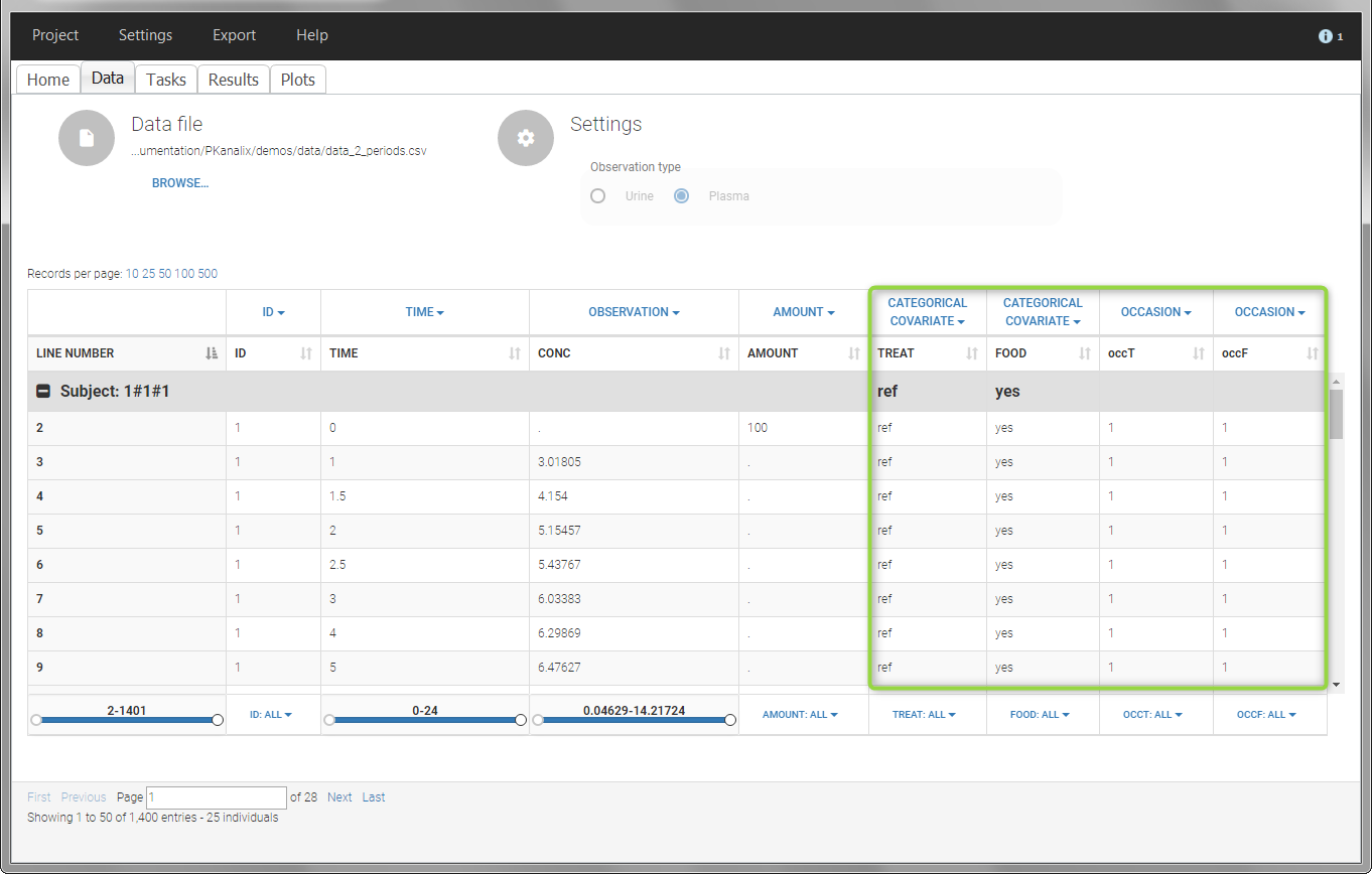
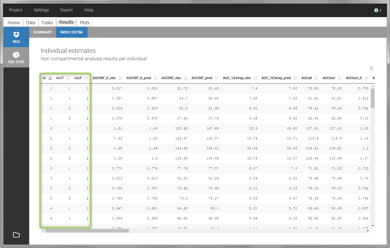
In the individual parameters tables and plots, three levels are visible. In the “Individual parameters vs covariates”, we can plot Cmax versus FOOD, split by TREAT for instance (Cmax versus TREAT split by FOOD is also possible).
 |
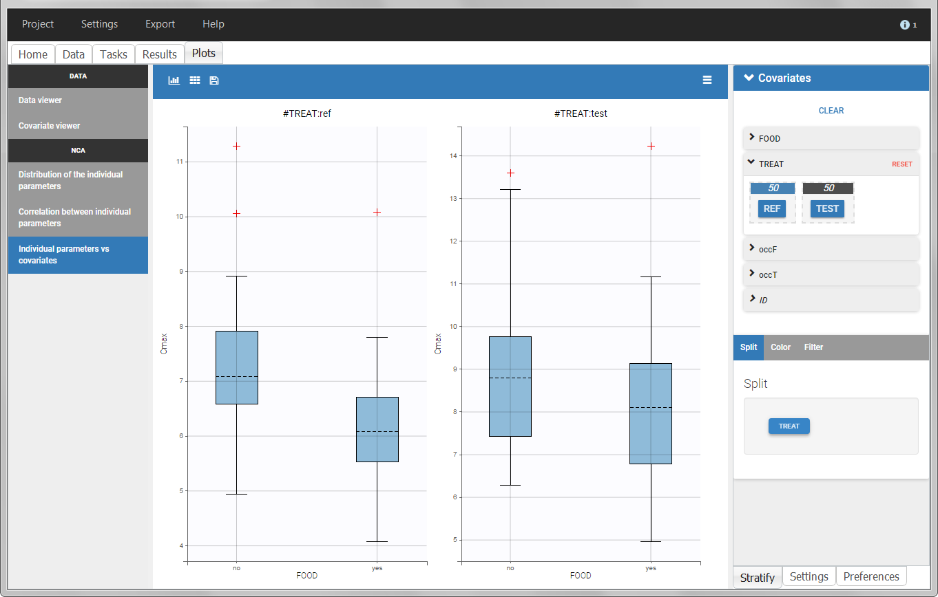 |
Covariates (“Carry” variables)
Individual information that need to be carried over to output tables and plots must be tagged as CATEGORICAL or CONTINUOUS COVARIATES. Categorical covariates define variables with a few categories, such as treatment or sex, and are encoded as strings. Continuous covariates define variables on a continuous scale, such as weight or age, and are encoded as numbers. Covariates will not automatically be used as “Sort” variables. A dedicated OCCASION column is necessary (see above).
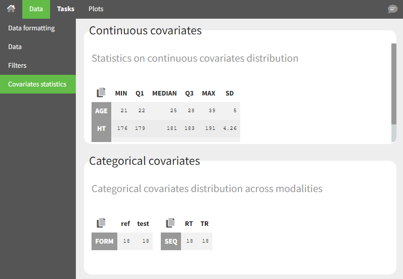
Covariates will automatically appear in the output tables. Plots of estimated NCA and/or CA parameters versus covariate values will also be generated. In addition, covariates can be used to stratify (split, color or filter) any plot. Statistics about the covariates distributions are available in table format in “Results > Cov. stat.” and in graphical format in “Plots > Covariate viewer”.
Note: It is preferable to avoid spaces and special characters (stars, etc) in the strings for the categories of the categorical covariates. Underscores are allowed.
Example:
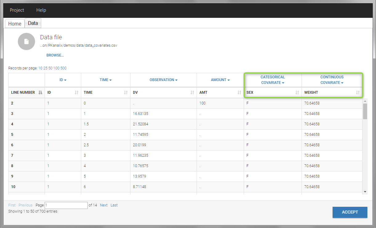
- demo project_covariates.pkx
In this data set, “SEX” is tagged as CATEGORICAL COVARIATE and “WEIGHT” as CONTINUOUS COVARIATE.
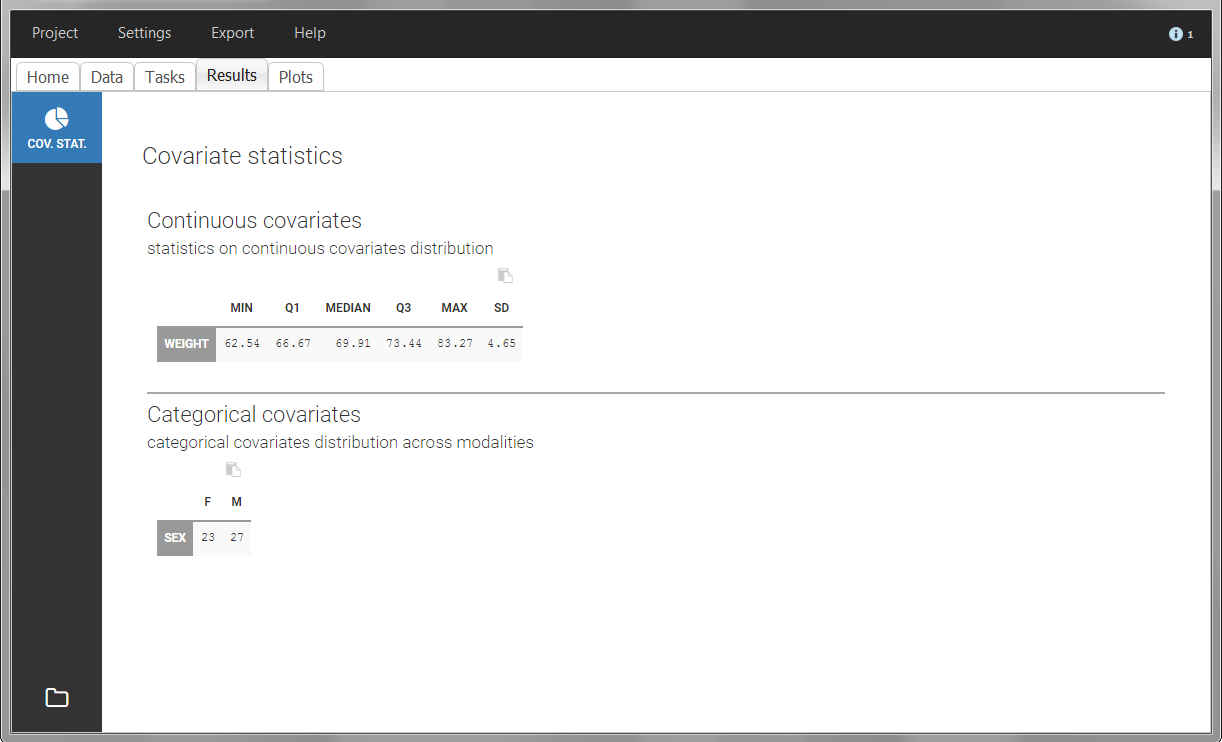
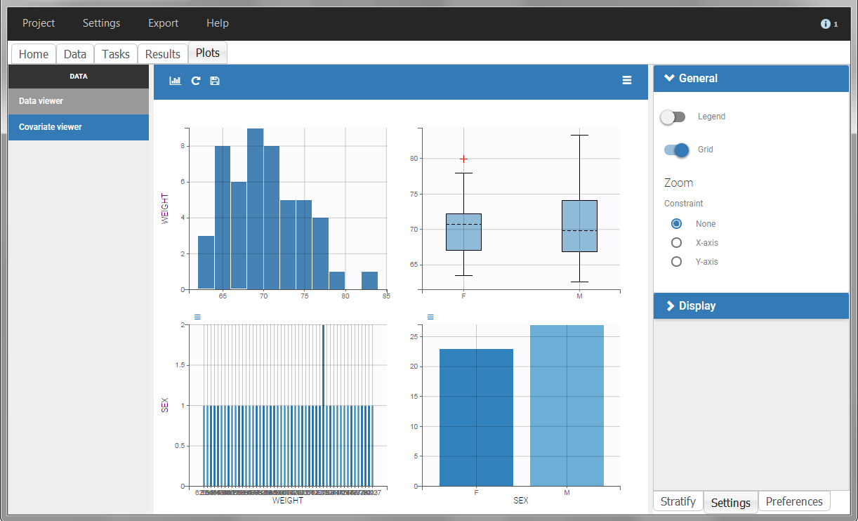
The “cov stat” table permits to see a few statistics of the covariate values in the data set. In the plot “Covariate viewer”, we see that the distribution of weight is similar for males and females.
 |
 |
After running the NCA and CA tasks, both covariates appear in the table of individual estimated parameters estimated.
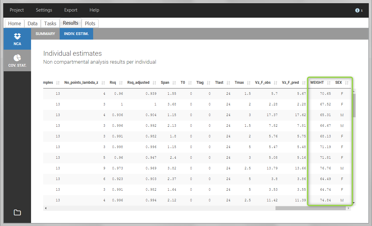
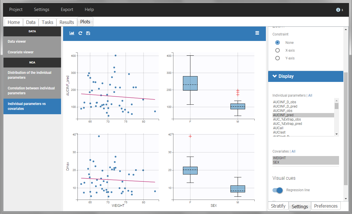
In the plot “parameters versus covariates”, the parameters values are plotted as scatter plot with the parameter value (here Cmax and AUCINF_pred) on on y-axis and the weight value on the x-axis, and as boxplots for sex female and sex male.
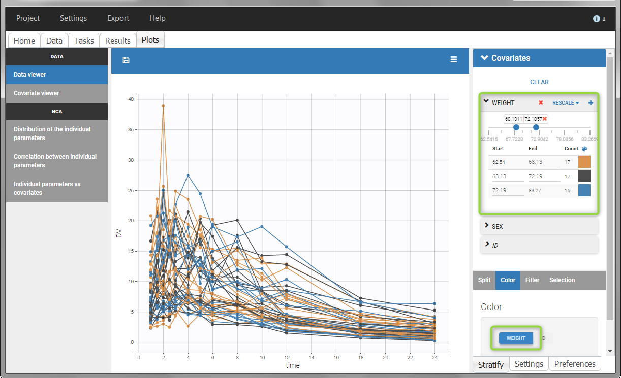
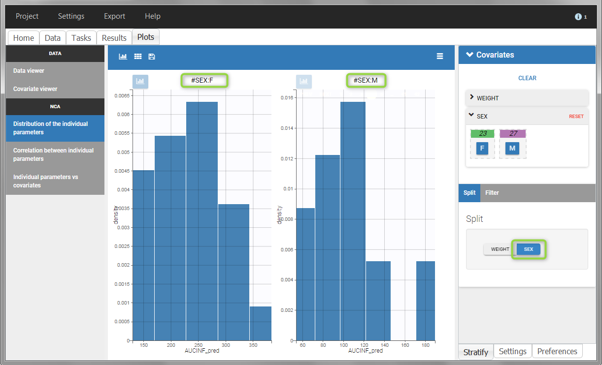
All plots can be stratified using the covariates. For instance, the “Data viewer” can be colored by weight after having created 3 weight groups. Below we also show the plot “Distribution of the parameters” split by sex with selection of the AUCINF_pred parameter.
 |
 |
Description of all possible column types
Column-types used for all types of lines:
- ID (mandatory): identifier of the individual
- OCCASION (formerly OCC): identifier (index) of the occasion
- TIME (mandatory): time of the dose or observation record
- NOMINAL TIME: time at which doses and observations were expected to occur
- DATE/DAT1/DAT2/DAT3: date of the dose or observation record, to be used in combination with the TIME column
- EVENT ID (formerly EVID): identifier to indicate if the line is a dose-line or a response-line
- IGNORED OBSERVATION (formerly MDV): identifier to ignore the OBSERVATION information of that line
- IGNORED LINE (from 2019 version): identifier to ignore all the informations of that line
- CONTINUOUS COVARIATE (formerly COV): continuous covariates (which can take values on a continuous scale)
- CATEGORICAL COVARIATE (formerly CAT): categorical covariate (which can only take a finite number of values)
- REGRESSOR (formerly X): defines a regression variable, i.e a variable that can be used in the structural model (used e.g for time-varying covariates)
- IGNORE: ignores the information of that column for all lines
Column-types used for response-lines:
- OBSERVATION (mandatory, formerly Y): records the measurement/observation for continuous, count, categorical or time-to-event data
- OBSERVATION ID (formerly YTYPE): identifier for the observation type (to distinguish different types of observations, e.g PK and PD)
- CENSORING (formerly CENS): marks censored data, below the lower limit or above the upper limit of quantification
- LIMIT: upper or lower boundary for the censoring interval in case of CENSORING column
Column-types used for dose-lines:
- AMOUNT (mandatory, formerly AMT): dose amount (with version 2024 only mandatory if dataset contains STEADY STATE, ADDITIONAL DOSES, INFUSIONRATE or INFUSION DURATION columns)
- ADMINISTRATION ID (formerly ADM): identifier for the type of dose (given via different routes for instance)
- INFUSION RATE (formerly RATE): rate of the dose administration (used in particular for infusions)
- INFUSION DURATION (formerly TINF): duration of the dose administration (used in particular for infusions)
- ADDITIONAL DOSES (formerly ADDL): number of doses to add in addition to the defined dose, at intervals INTERDOSE INTERVAL
- INTERDOSE INTERVAL (formerly II): interdose interval for doses added using ADDITIONAL DOSES or STEADY-STATE column types
- STEADY STATE (formerly SS): marks that steady-state has been achieved, and will add a predefined number of doses before the actual dose, at interval INTERDOSE INTERVAL, in order to achieve steady-state
2.3.Data formatting
The dataset format that is used in PKanalix is the same as for the entire MonolixSuite, to allow smooth transitions between applications. In this format, some rules have to be fullfilled, for example:
- Each line corresponds to one individual and one time point.
- Each line can include a single measurement (also called observation), or a dose amount (or both a measurement and a dose amount).
- Dose amount should be indicated for each individual dose in a column AMOUNT, even if it is identical for all.
- Headers are free but there can be only one header line.
If your dataset is not in this format, in most cases, it is possible to format it in a few steps in the data formatting tab, to incorporate the missing information.
In this case, the original dataset should be loaded in the “Format data” box, or directly in the “Data Formatting” tab, instead of the “Data” tab. In the data formatting module, you will be guided to build a dataset in the MonolixSuite format, starting from the loaded csv file. The resulting formatted dataset is then loaded in the Data tab as if you loaded an already-formatted dataset in “Data” directly. Then as for defining any dataset, you can tag columns, accept the dataset, and once accepted, units can be specified in the Data tab and the Filters tab can be used to select only parts of this dataset for analysis. Note that units and filters are neither information to be included in the data file, nor part of the data formatting process.
From the version 2024R1, it is possible to save and reapply data formatting steps on multiple projects, using data formatting presets.
Jump to:
- Data formatting workflow
- Dataset initialization (mandatory step)
- Selecting header lines or lines to exclude to merge header lines or exclude a line
- Tagging mandatory columns such as ID and TIME
- Initialization example Demo project CreateOcc_AdmIdbyCategory.pkx
- Creating occasions from a SORT column to distinguish different sets of measurements within each subject, (eg formulations). Demo project CreateOcc_AdmIdbyCategory.pkx
- Selecting an observation type (required to add a treatment)
- Merging observations from several columns
- As observation ids to map them to several outputs in CA. Demo project merge_obsID_ParentMetabolite.pkx
- As occasions to analyze them simultaneously in NCA. Demo project merge_occ_ParentMetabolite.pkx
- Option “Duplicate information from undefined columns”
- Specifying censoring from censoring tags eg “BLQ” instead of a number in an observation column. Demo project DoseAndLOQ_manual.pkx
- Adding doses in the dataset Demo project DoseAndLOQ_manual.pkx
- Reading censoring limits or dosing information from the dataset “by category” or “from data”. Demo projects DoseAndLOQ_byCategory.pkx and DoseAndLOQ_fromData.pkx
- Creating occasions from dosing intervals to analyze separately the measurements following different doses.Demo project doseIntervals_as_Occ.mlxtran
- Handling urine data to merge start and end times in a single column. Demo project Urine_LOQinObs.pkx
- Adding new columns from an external file, eg new covariates, or individual parameters estimated in a previous analysis. Demo warfarin_PKPDseq_project.mlxtran
- Exporting the formatted dataset
1. Data formatting workflow
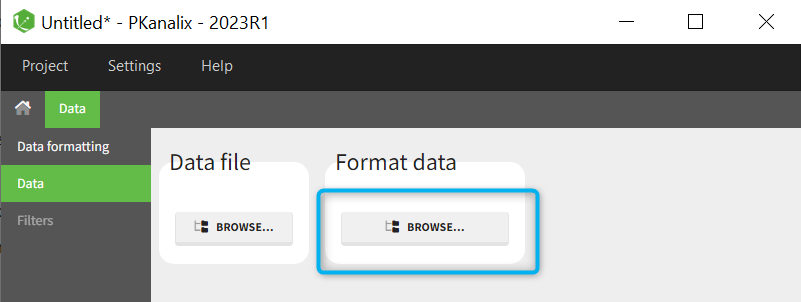
When opening a new project, two Browse buttons appear. The first one, under “Data file”, can be used to load a dataset already in a MonolixSuite-standard format, while the second one, under “Format data”, allows to load a dataset to format in the Data formatting module.
After loading a dataset to format, data formatting operations can be specified in several subtabs: Initialization, Observations, Treatments and Additional columns.
- Initialization is mandatory and must be filled before using the other subtabs.
- Observations is required to enable the Treatments tab.
After Initialization has been validated by clicking on “Next”, a button “Preview” is available from any subtab to view in the Data tab the formatted dataset based on the formatting operations currently specified.

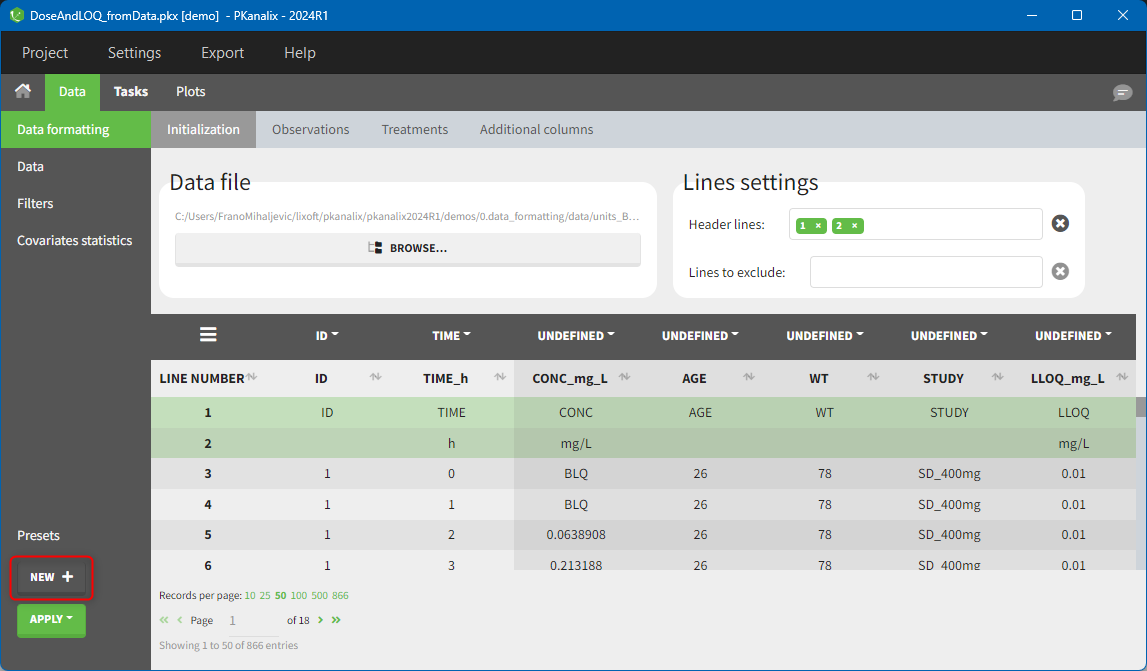
2. Dataset initialization
The first tab in Data formatting is named Initialization. This is where the user can select header lines or lines to exclude (in the blue area on the screenshot below) or tag columns (in the yellow area).
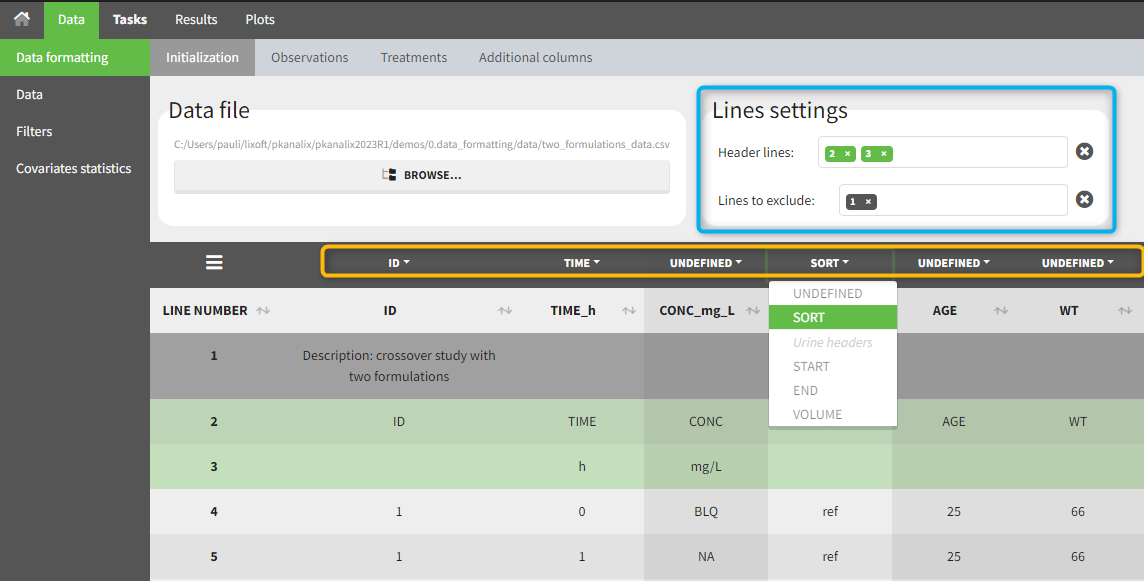
Selecting header lines or lines to exclude
These settings should contain line numbers for lines that should be either handled as column headers or that should be excluded.
- Header lines: one or several lines containing column header information. By default, the first line of the dataset is selected as header. If several lines are selected, they are merged by data formatting into a single line, concatenating the cells in each column.
- Lines to exclude (optional): lines that should be excluded from the formatted dataset by data formatting.
Tagging mandatory columns
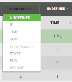
Only the columns corresponding to the following tabs must be tagged in Initialization, while all the other columns should keep the default UNDEFINED tag:
- ID (mandatory): subject identifiers
- TIME (mandatory): the single time column
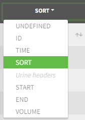
- SORT (optional): one or several columns containing SORT variables can be tagged as SORT. Occasions based on these columns will be created in the formatted dataset as described in Section 3.
- START, END and VOLUME (mandatory in case of urine data): these column tags replace the TIME tag in case of urine data, if the urine collection time intervals are encoded in the dataset with two time columns for the start and end times of the intervals. In that case there should also be a column with the urine volume in each interval. See Section 10 for more details.
Initialization example
- demo CreateOcc_AdmIdbyCategory.pkx (the screenshot below focuses on the formatting initialization and excludes other elements present in the demo):
In this demo the first line of the dataset is excluded because it contains a description of the study. The second line contains column headers while the third line contains column units. Since the MonolixSuite-standard format allows only a single header line, lines 2 and 3 are merged together in the formatted dataset.
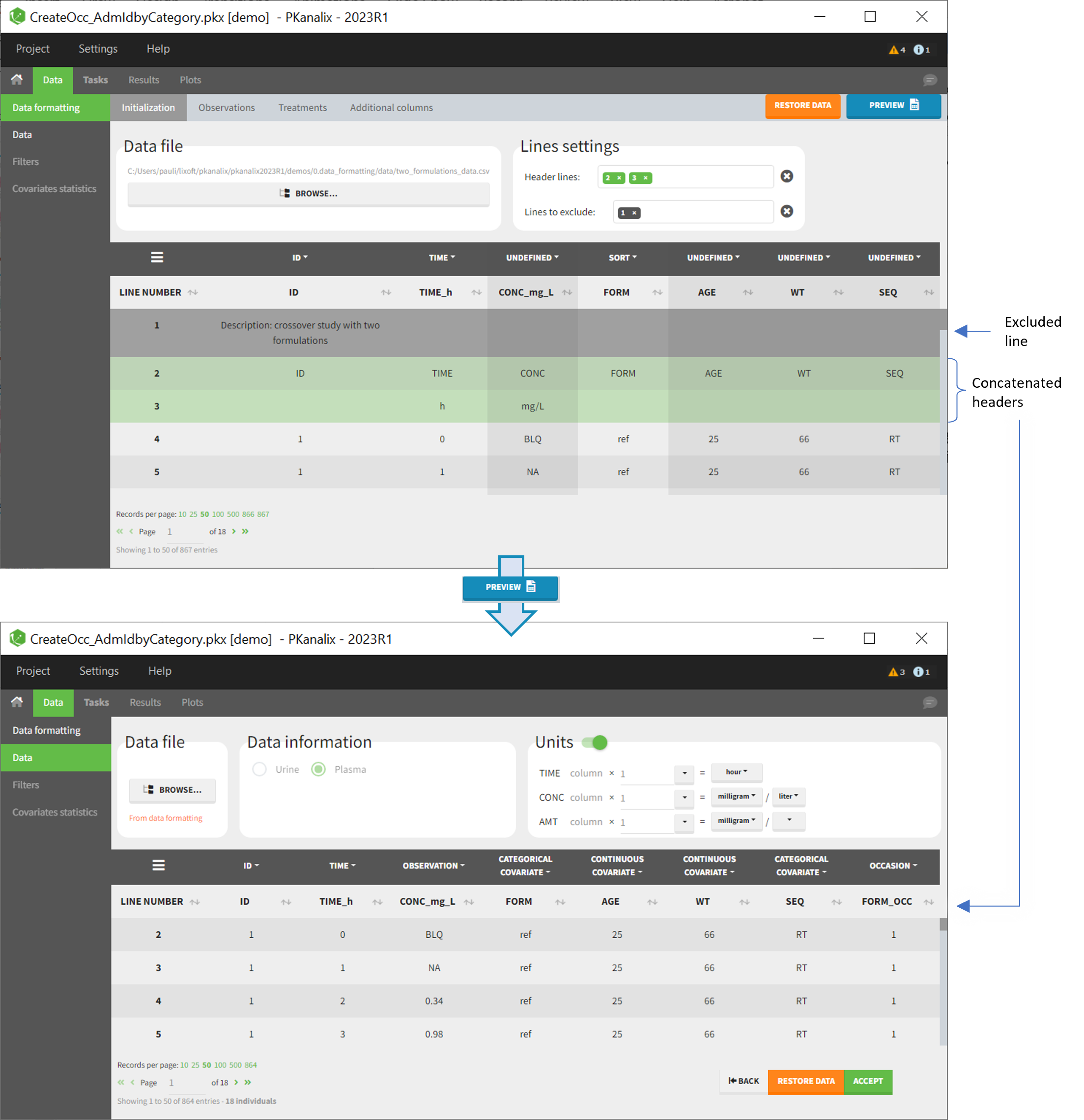
3. Creating occasions from a SORT column
A SORT variable can be used to distinguish different sets of measurements (usually concentrations) within each subject, that should be analyzed separately by PKanalix (for example: different formulations given to each individual at different periods of time, or multiple doses where concentration profiles are available to be analyzed following several doses).
In PKanalix, these different sets of measurements must be distinguished as OCCASIONS (or periods of time), via the OCCASION column-type. However, a column tagged as OCCASION can only contain integers with occasion indexes. Thus, if a column with a SORT variable contains strings, its format must be adapted by Data formatting, in the following way:
- the user must tag the column as SORT in the Initialization subtab of Data formatting,
- the user validates the Initialization with “Next”, then clicks on “Preview” (after optionally defining other data formatting operations),
- the formatted data is shown in Data: the column tagged as SORT is automatically duplicated. The original column is automatically tagged as CATEGORICAL COVARIATE in Data, while the duplicated column, which has the same name appended with “_OCC”, is tagged as OCCASION. This column contains occasion indexes instead of strings.
Example:
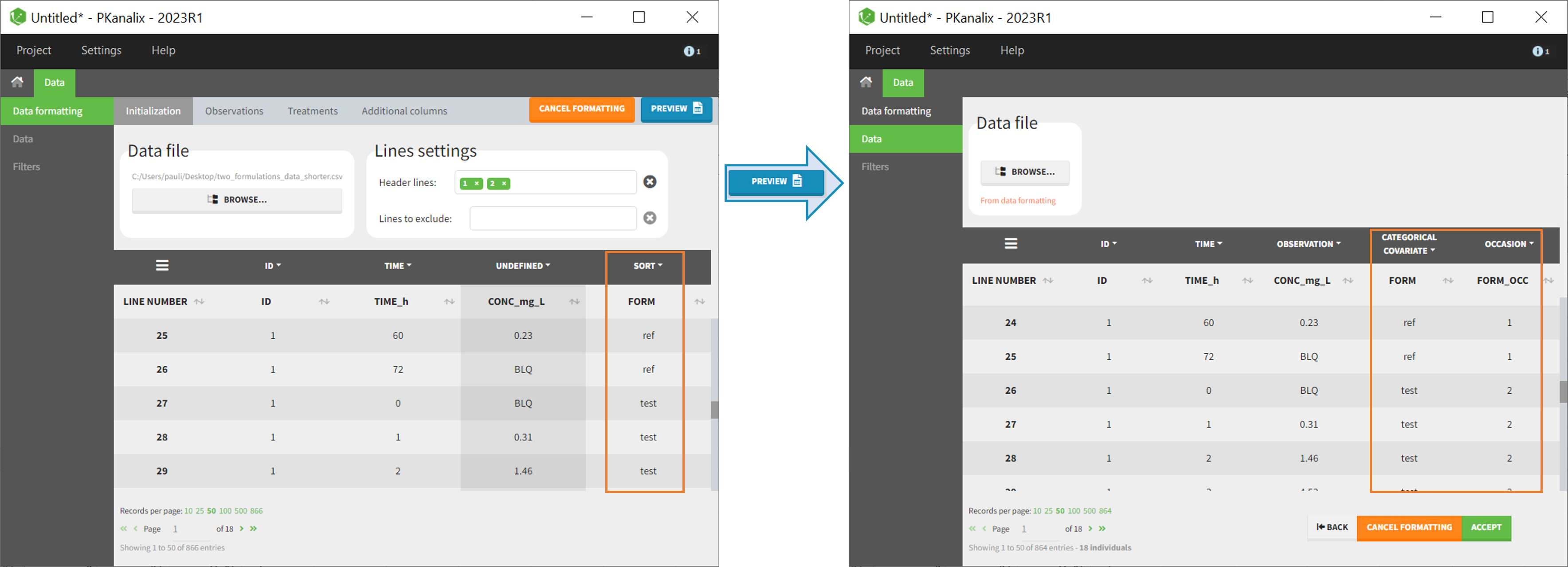
- demo CreateOcc_AdmIdbyCategory.pkx (the screenshot below focuses on the formatting of occasions and excludes other elements present in the demo):
The image below shows lines 25 to 29 from the dataset from the CreateOcc_AdmIdbyCategory.pkx demo, where covariate columns have been removed to simplify the example. This dataset contains two sets of concentration measurements for each individual, corresponding to two different drug formulations administered on different periods. The sets of concentrations are distinguished with the FORM column, which contains “ref” and “test” categories (reference/test formulations). The column is tagged as SORT in Data formatting Initialization. After clicking on “Preview”, we can see in the Data tab that a new column named FORM_OCC has been created with occasion indexes for each individual: for subject 1, FORM_OCC=1 corresponds to the reference formulation because it appears first in the dataset, and FORM_OCC=2 corresponds to the test formulation because it appears in second in the dataset.
4. Selecting an observation type
The second subtab in Data formatting allows to select one or several observation types. An observation type corresponds to a column of the dataset, that contains a type of measurements (usually drug concentrations, but it can also be PD measurements for example). Only columns that have not been tagged as ID, TIME or SORT are available as observation type.
This action is optional and can have several purposes:
- If doses must be added by Data formatting (see Section 7), specifying the column containing observations is mandatory, to avoid duplicating observations on new dose lines.
- If several observation types exist in different columns (for example: concentrations for different analytes, or measurements for PK and PD), they must be specified in Data formatting to be merged into a single observation column (see Section 5).
- In the MonolixSuite-standard format, the column containing observations can only contain numbers, and no string except “.” for a missing observation. Thus if this column contains strings in the original dataset, it must be adapted by Data formatting, with two different cases:
- if the strings are tags for censored observations (usually BLQ: below the limit of quantification), they can be specified in Data formatting to adapt the encoding of the censored observations (see Section 6),
- any other string in the column is automatically replaced by “.” by Data formatting.
5. Merging observations from several columns
The MonolixSuite-standard format allows a single column containing all observations (such as concentrations or PD measurements). Thus if a dataset contains several observation types in different columns (for example: concentrations for different analytes, or measurements for PK and PD), they must be specified in Data formatting to be merged into a single observation column.
In that case, different settings can be chosen in the area marked in orange in the screenshot below:
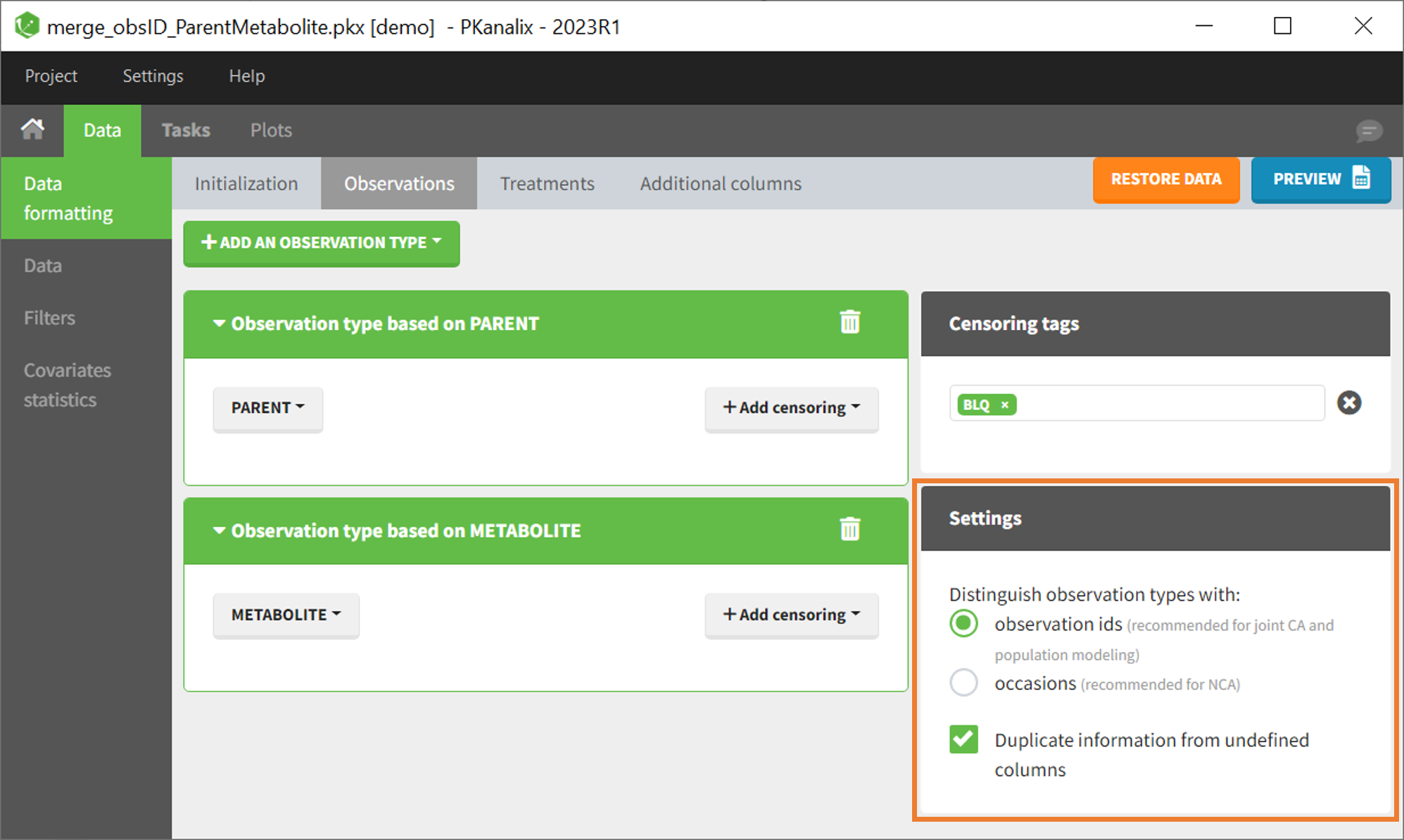
- The user must choose between distinguishing observation types with observation ids or occasions.
- The user can unselect the option “Duplicate information from undefined columns”.
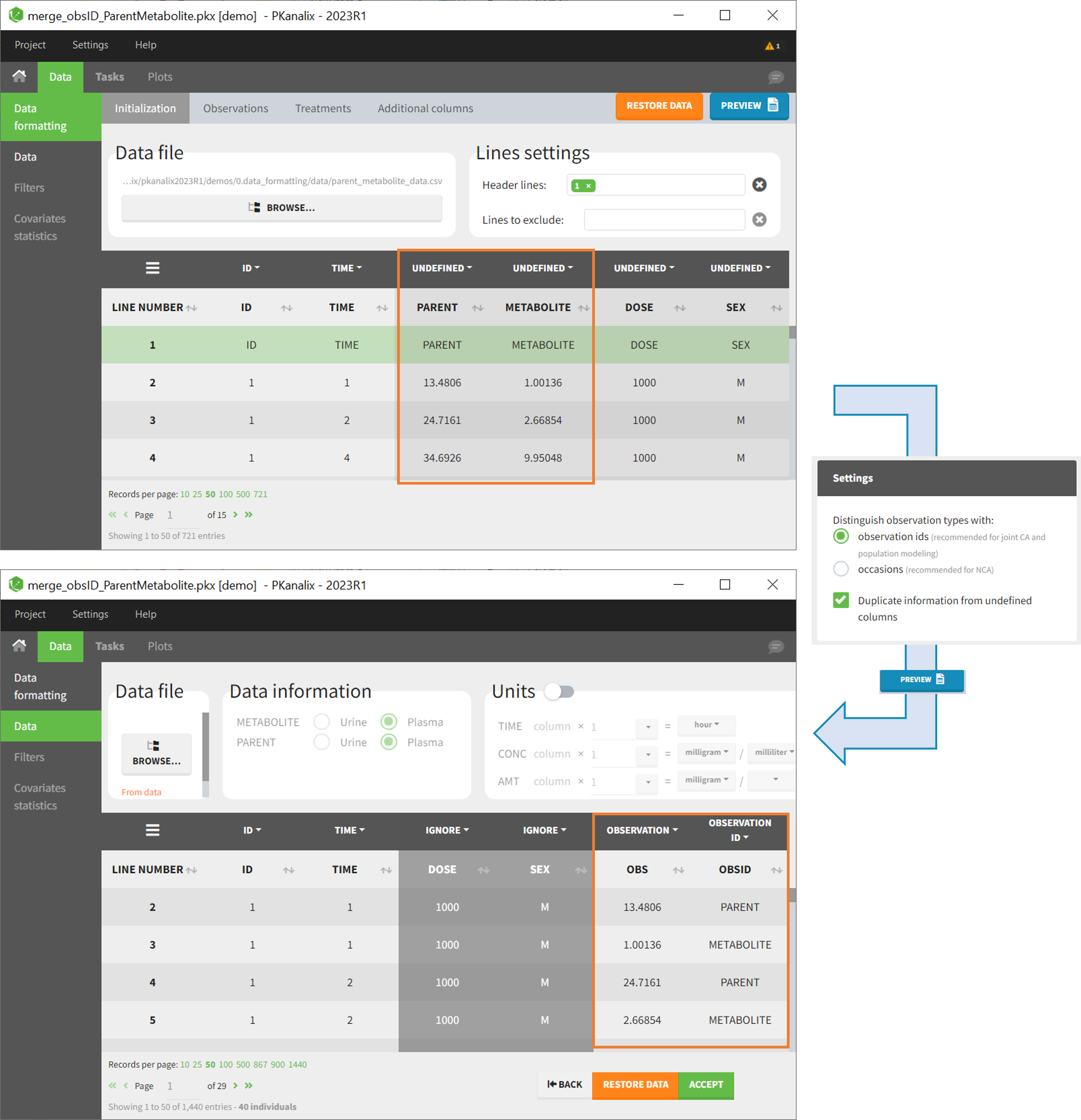
As observation ids
After selecting the “Distinguish observation types with: observation ids” option and clicking “Preview,” the columns for different observation types are combined into a single column called “OBS.” Each row of the dataset is duplicated for each observation type, with one value per observation type. Additionally, an “OBSID” column is created, with the name of the observation type corresponding to the measurement on each row.
This option is recommended for joint modeling of observation types, such as CA in PKanalix or population modeling in Monolix. It is important to note that NCA cannot be performed on two different observation ids simultaneously, so it is necessary to choose one observation id for the analysis.
Example:
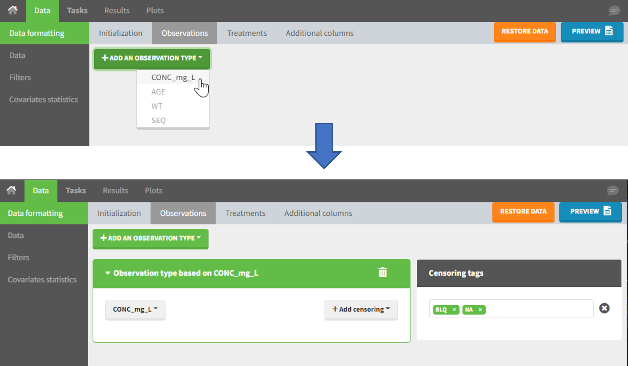
- demo merge_obsID_ParentMetabolite.pkx (the screenshot below focuses on the formatting of observations and excludes other elements present in the demo):
This demo involves two columns that contain drug parent and metabolite concentrations. When merging both observation types with observation ids, a new column called OBSID is generated with categories labeled as “PARENT” and “METABOLITE.”
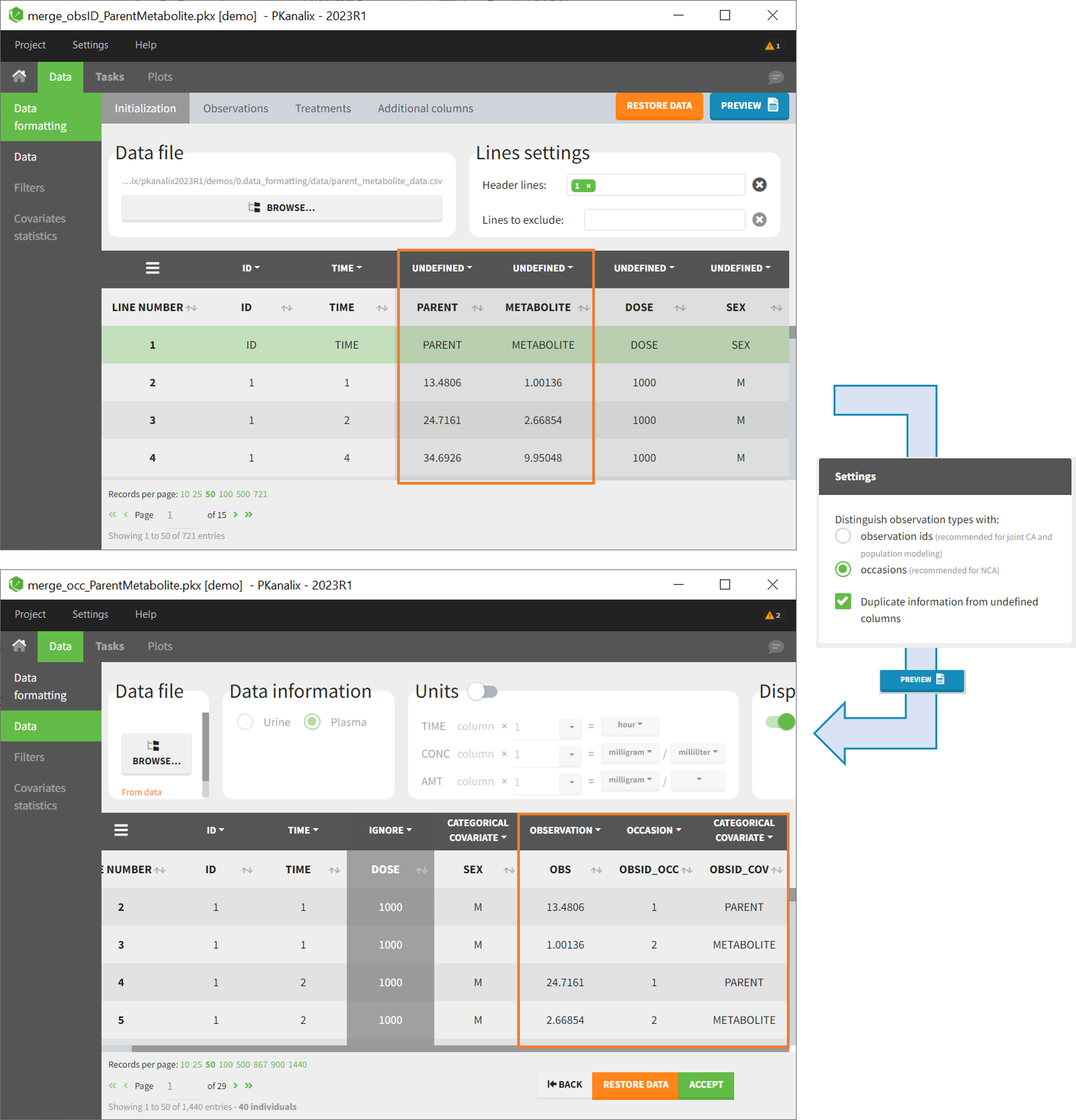
As occasions
After selecting the “Distinguish observation types with: occasions” option and clicking “Preview,” the columns for different observation types are combined into a single column called “OBS.” Each row of the dataset is duplicated for each observation type, with one value per observation type. Additionally, two columns are created: an “OBSID_OCC” column with the index of the observation type corresponding to the measurement on each row, and an “OBSID_COV” with the name of the observation type.
This option is recommended for NCA, which can be run on different occasions for each individual. However, joint modeling of the observation types with CA or population modeling with Monolix cannot be performed with this option.
Example:
- demo merge_occ_ParentMetabolite.pkx:
This demo involves two columns that contain drug parent and metabolite concentrations. When merging both observation types with occasions, two new columns called OBSID_OCC and OBSID_COV are generated with OBSID_OCC=1 corresponding to OBSID_COV=”PARENT” catand OBSID_OCC=2 corresponding to OBSID_COV=”METABOLITE.”
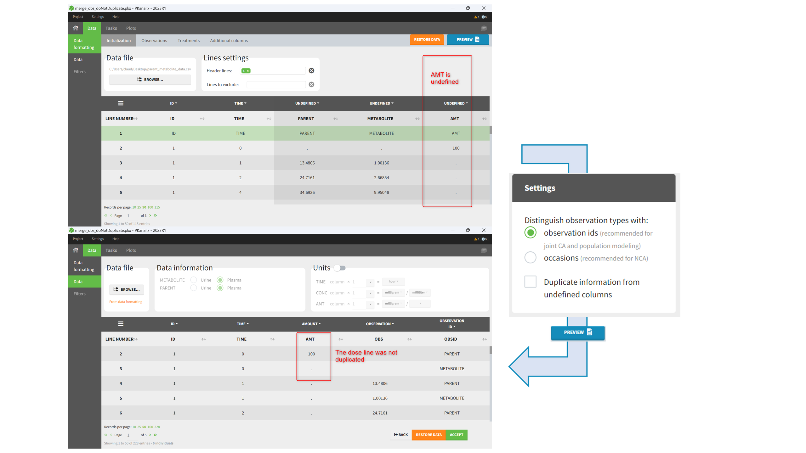
Duplicate information from undefined columns
When merging two observation columns into a single column, all other columns will see their lines duplicated. The data formatting will know how to treat columns which have been tagged in the Initialization tab, but not the other columns (header “UNDEFINED”) which are not used for data formatting. A checkbox enables to decide if the information from these columns should be duplicated on the new lines, or if “.” should be used instead. The default option is to duplicate information, because in general, the undefined columns correspond to covariates with one value per individual, so this value is the same for the two lines that correspond to the same id.
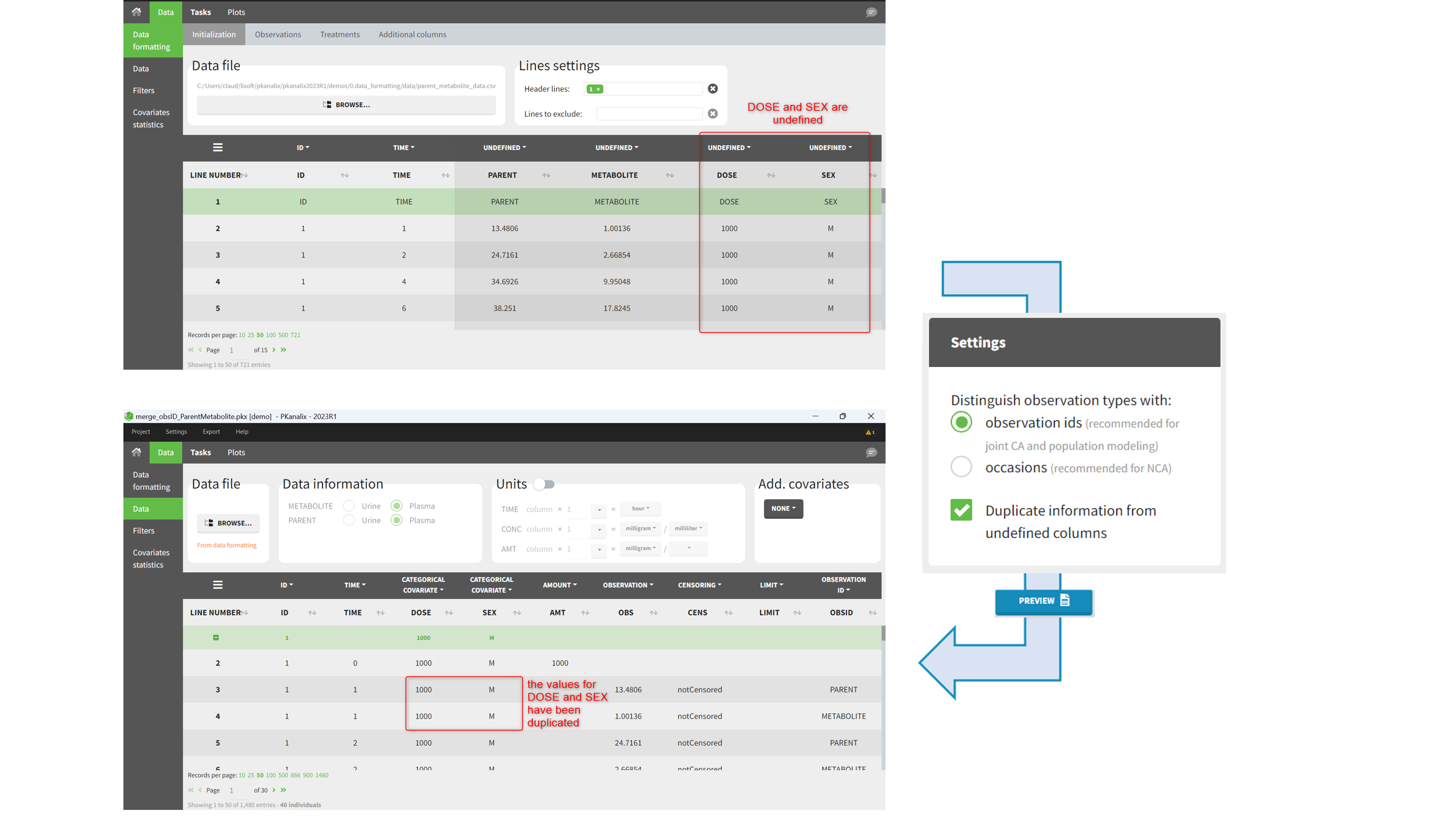
It is rare that you need to uncheck this box. An example where you should not duplicate the information is if you already have a column Amount in the MonolixSuite format, so with a dose amount only at the dosing time, and “.” everywhere else. If you do not want to specify amount again in data formatting, and simply want to merge observation columns as observation ids, you should not duplicate the lines of the Amount column which is undefined. Indeed, the dose amounts have been administered only once.
6. Specifying censoring from censoring tags
In the MonolixSuite-standard format, censored observations are encoded with a 1or -1 flag in a column tagged as CENSORING in the Data tab, while exact observations have a 0 flag in that column. In addition, on rows for censored observations, the LOQ is indicated in the observation column: it is the LLOQ (lower limit of quantification) if CENSORING=1 or the ULOQ (upper limit of quantification) if CENSORING=-1. Finally, to specify a censoring interval, an additional column tagged as LIMIT in the Data tab must exist in the dataset, with the other censoring bound.
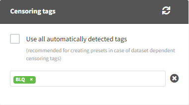
The Data Formatting module can take as input a dataset with censoring tags directly in the observation column, and adapt the dataset format as described above. After selecting one or several observation types in the Observations subtab (see Section 4), all strings found in the corresponding columns are displayed in the “Censoring tags” on the right of the observation types. If at least one string is found, the user can then define some censoring associated with an observation type and with one or several censoring tags with the button “Add censoring”. Additionally, option “Use all automatically detected tags” exist and can be used when all censoring tags correspond to the same censoring type (this option is recommended for the usage with data formatting presets, if censoring tags vary between data sets in which the preset will be used). 3 types of censoring can be defined:
- LLOQ: this corresponds to left-censoring, where the censored observation is below a lower limit of quantification (LLOQ), that must specified by the user. In that case Data Formatting replaces the censoring tags in the observation column by the LLOQ, and creates a new CENS column tagged as CENSORING in the Data tab, with 1 on rows that had censoring tags before formatting, and 0 on other rows.
- ULOQ: this corresponds to right-censoring, where the censored observation is above an upper limit of quantification (ULOQ), that must specified by the user. Here Data Formatting replaces the censoring tags in the observation column by the ULOQ, and creates a new CENS column tagged as CENSORING in the Data tab, with -1 on rows that had censoring tags before formatting, and 0 on other rows.
- Interval: this is for interval-censoring, where the user must specify two bound of a censoring interval, to which the censored observation belong. Data Formatting replaces the censoring tags in the observation column by the upper bound of the interval, and creates two new columns: a CENS column tagged as CENSORING in the Data tab, with 1 on rows that had censoring tags before formatting, and 0 on other rows, and a LIMIT column with the lower bound of the censoring interval on rows that had censoring tags before formatting, and “.” on other rows.
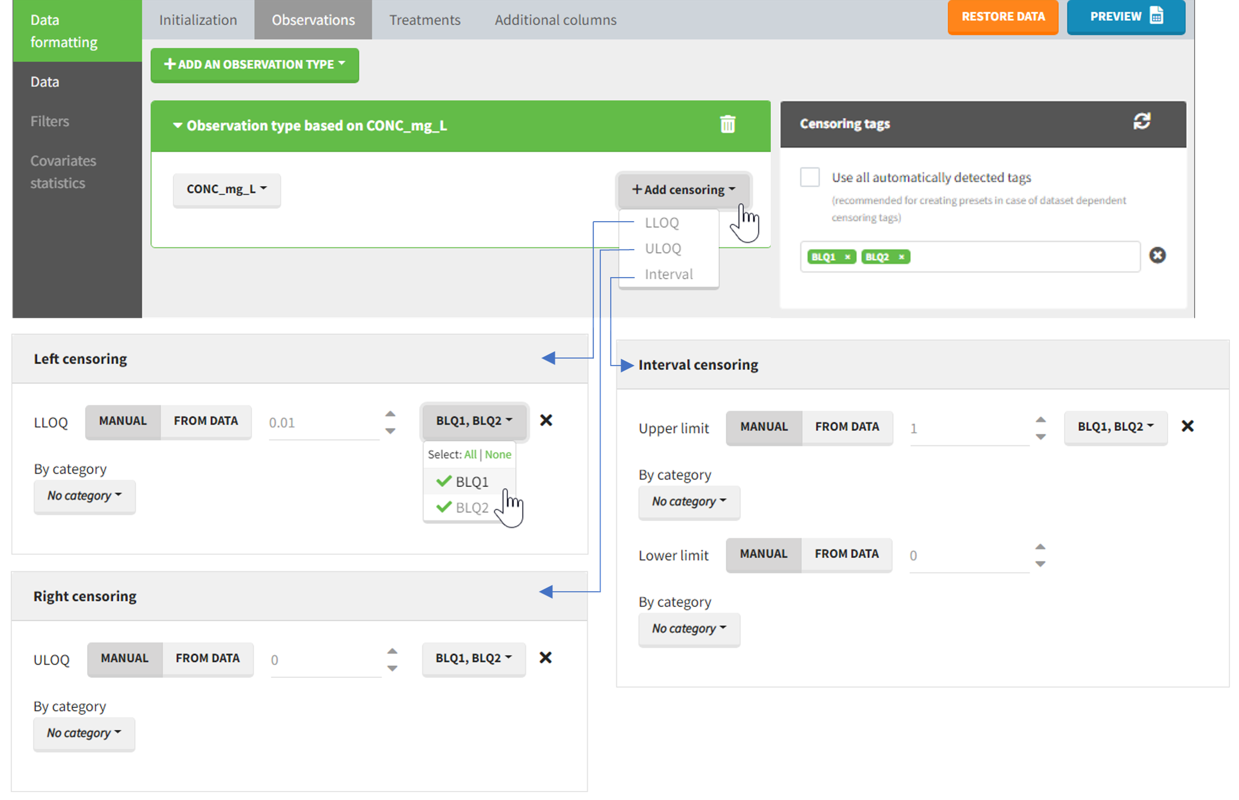
For each type of censoring, available options to define the limits are:
- “Manual“: limits are defined manually, by entering the limit values for all censored observations.
- “By category“: limits are defined manually for different categories read from the dataset.
- “From data“: limits are directly read from the dataset.
The options “by category” and “from data” are described in detail in Section 8.
Example:
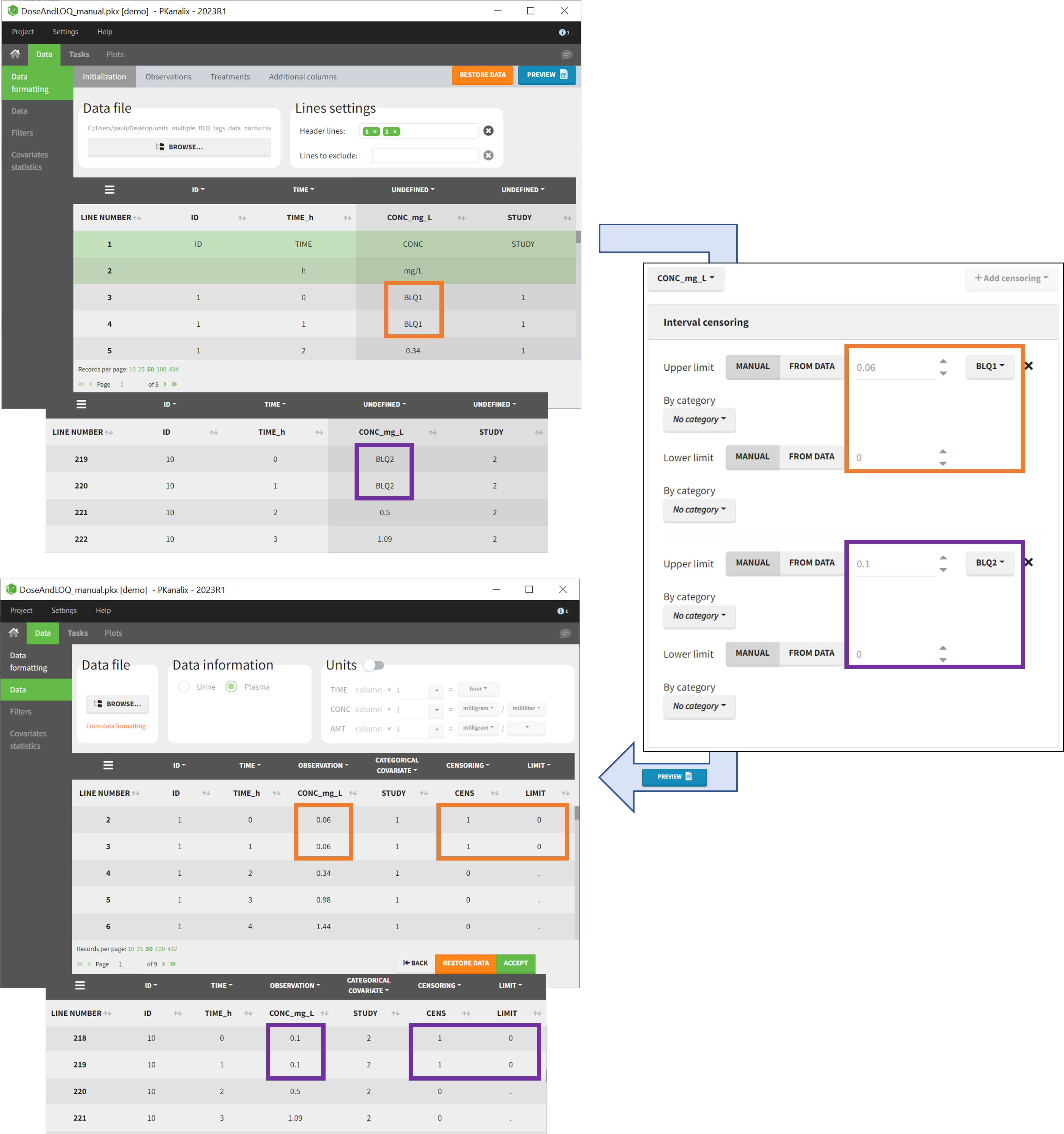
- demo DoseAndLOQ_manual.pkx (the screenshot below focuses on the formatting of censored observations and excludes other elements present in the demo):
In this demo there are two censoring tags in the CONC column: BLQ1 (from Study 1) and BLQ2 (from Study 2), that correspond to different LLOQs. An interval censoring is defined for each censoring tag, with manual limits, where LLOQ=0.06 for BLQ1 and LLOQ=0.1 for BLQ2, and the lower limit of the censoring interval being 0 in both cases.
7. Adding doses in the dataset
Datasets in MonolixSuite-standard format should contain all information on doses, as dose lines. An AMOUNT column records the amount of the administrated doses on dose-lines, with “.” on response-lines. In case of infusion, an INFUSION DURATION or INFUSION RATE column records the infusion duration or rate. If there are several types of administration, an ADMINISTRATION ID column can distinguish the different types of doses with integers.
If doses are missing from a dataset, the Data Formatting module can be used to add dose lines and dose-related columns: after initializing the dataset, the user can specify one or several treatments in the Treatments subtab. The following operations are then performed by Data Formatting:
- a new dose line is inserted in the dataset for each defined dose, with the dataset sorted by subject and times. On such a dose line, the values from the next line are duplicated for all columns, except for the observation column in which “.” is used for the dose line.
- A new column AMT is created with “.” on all lines except on dose lines, on which dose amounts are used. The AMT column is automatically tagged as AMOUNT in the Data tab.
- If administration ids have been defined in the treatment, an ADMID column is created, with “.” on all lines except on dose lines, on which administration ids are used. The ADMID column is automatically tagged as ADMINISTRATION ID in the Data tab.
- If an infusion duration or rate has been defined, a new INFDUR (for infusion duration) or INFRATE (for infusion rate) is created, with “.” on all lines except on dose lines. The INFDUR column is automatically tagged as INFUSION DURATION in the Data tab, and the INFRATE column is automatically tagged as INFUSION RATE.
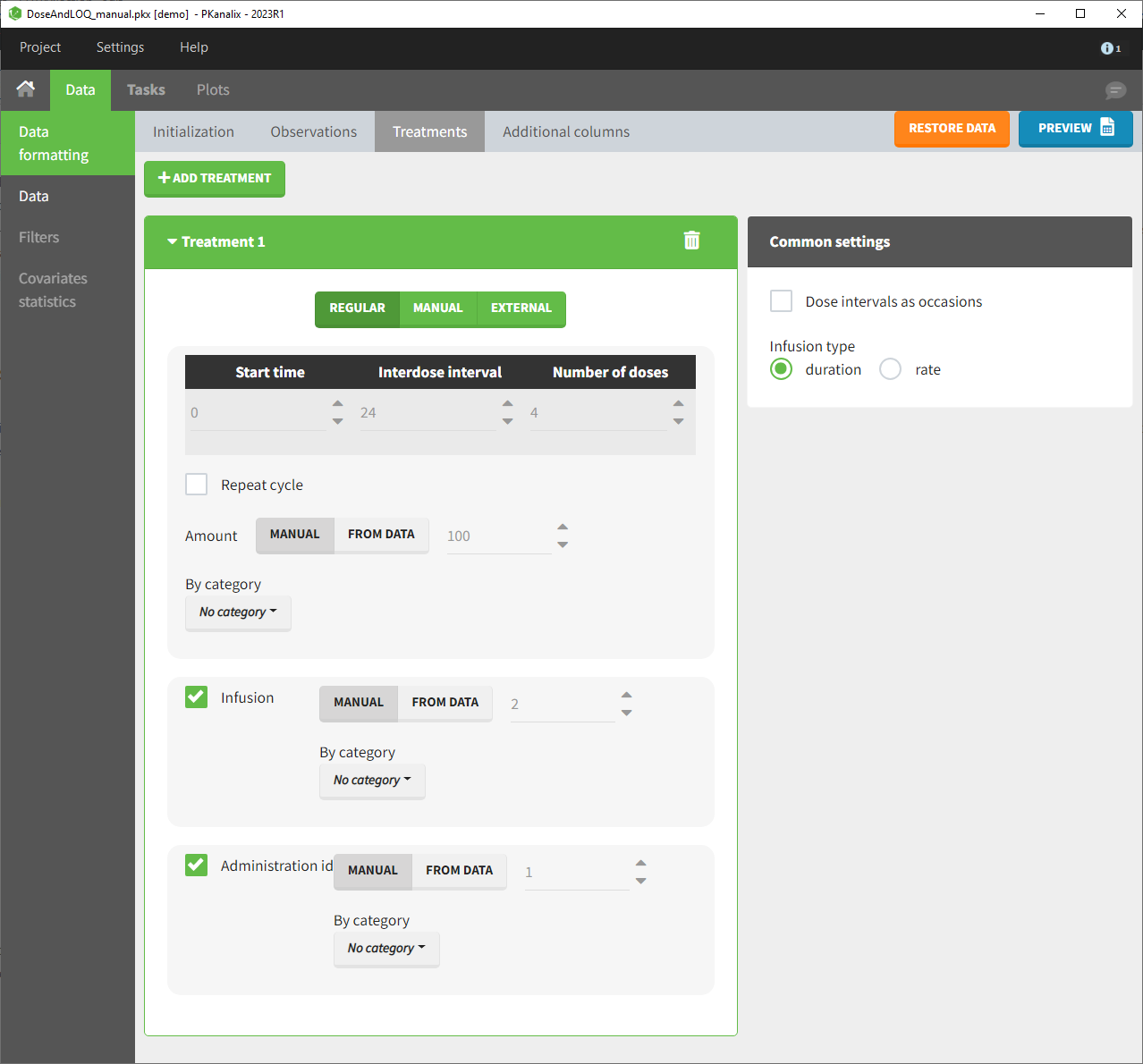
For each treatment, the dosing schedule can defined as:
- regular: for regularly spaced dosing times, defined with the start time, inter-dose internal, and number of doses. A “repeat cycle” option allows to repeat the regular dosing schedule to generate a more complex regimen.
- manual: a vector of one or several dosing times, each defined manually. A “repeat cycle” option allows to repeat the manual dosing schedule to generate a more complex regimen.
- external: an external text file with columns id (optional), occasions (optional), time (mandatory), amount (mandatory), admid (administration id, optional), tinf or rate (optional), that allows to define individual doses.
Starting from the 2024R1 version, different dosing schedules can be defined for different individuals, based on information from other columns, which can be useful in cases when different cohorts received different dosing regimens, or when working with data pooled from multiple studies. To define a treatment just for a specific cohort or study, the dropdown on the top of the treatment section can be used:

While dose amounts, administration ids and infusion durations or rates are defined in the external file for external treatments, available options to define them for treatments of type “manual” or “regular” are:
- “Manual“: this applies the same amount (or administration id or infusion duration or rate) to all doses.
- “By category“: dose amounts (or administration id or infusion duration or rate) are defined manually for different categories read from the dataset.
- “From data“: dose amounts (or administration id or infusion duration or rate) are directly read from the dataset.
The options “by category” and “from data” are described in detail in Section 8.
There is a “common settings” panel on the right:
- dose intervals as occasions: this creates a column to distinguish the dose intervals as different occasions (see Section 9).
- infusion type: If several treatments correspond to infusion administration, they need to share the same type of encoding for infusion information: as infusion duration or as infusion rate.
Example:
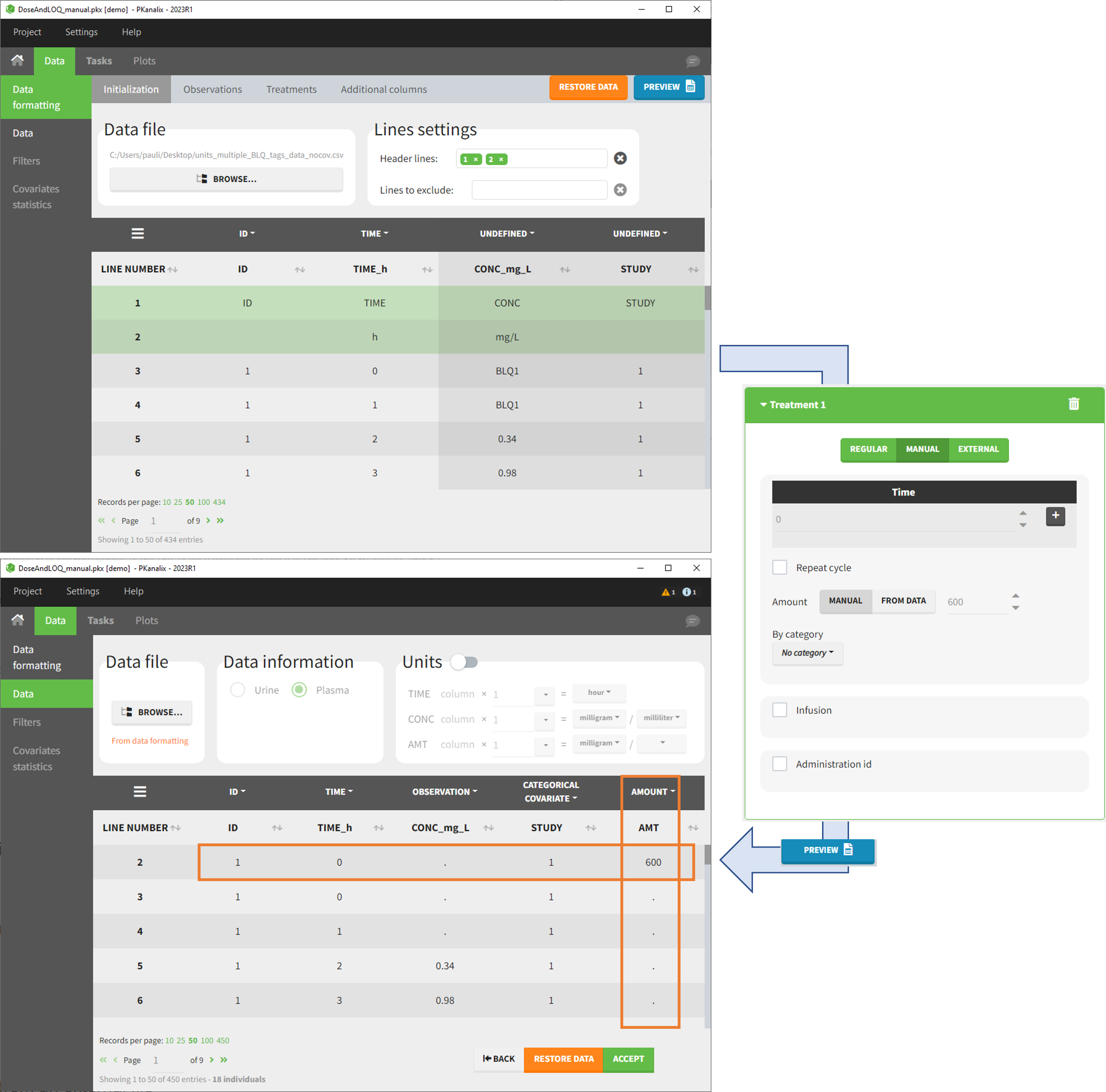
- demo DoseAndLOQ_manual.pkx (the screenshot below focuses on the formatting of doses and excludes other elements present in the demo):
In this demo, doses are initially not included in the dataset to format. A single dose at time 0 with an amount of 600 is added for each individual by Data Formatting. This creates a new AMT column in the formatted dataset, tagged as AMOUNT.
8. Reading censoring limits or dosing information from the dataset
When defining censoring limits for observations (see Section 6) or dose amounts, administration ids, infusion duration or rate for treatments (see Section 7), two options allow to define different values for different rows, based on information already present in the dataset: “by category” and “from data”.
By category
It is possible to define manually different censoring limits, dose amounts, administration ids, infusion durations, or rates for different categories within a dataset’s column. After selecting this column in the “By category” drop-down menu, the different modalities in the column are displayed and a value must be manually assigned each modality.
- For censoring limits, the censoring limit used to replace each censoring tag depends on the modality on the same row.
- For doses, the value chosen for the newly created column (AMT for amount, ADMID for administration id, INFDUR for infusion duration, INFRATE for infusion rate) on each new dose line depends on the modality on the first row found in the dataset for the same individual and the same time as the dose, or the next time if there is no line in the initial dataset at that time, or the previous time if no time is found after the dose.
Example:
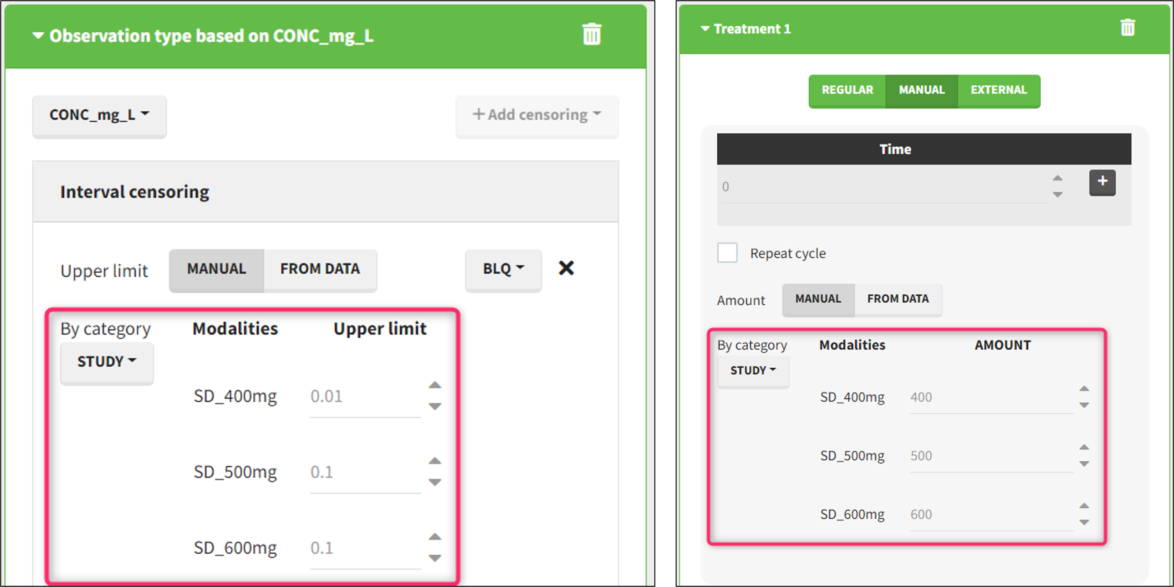
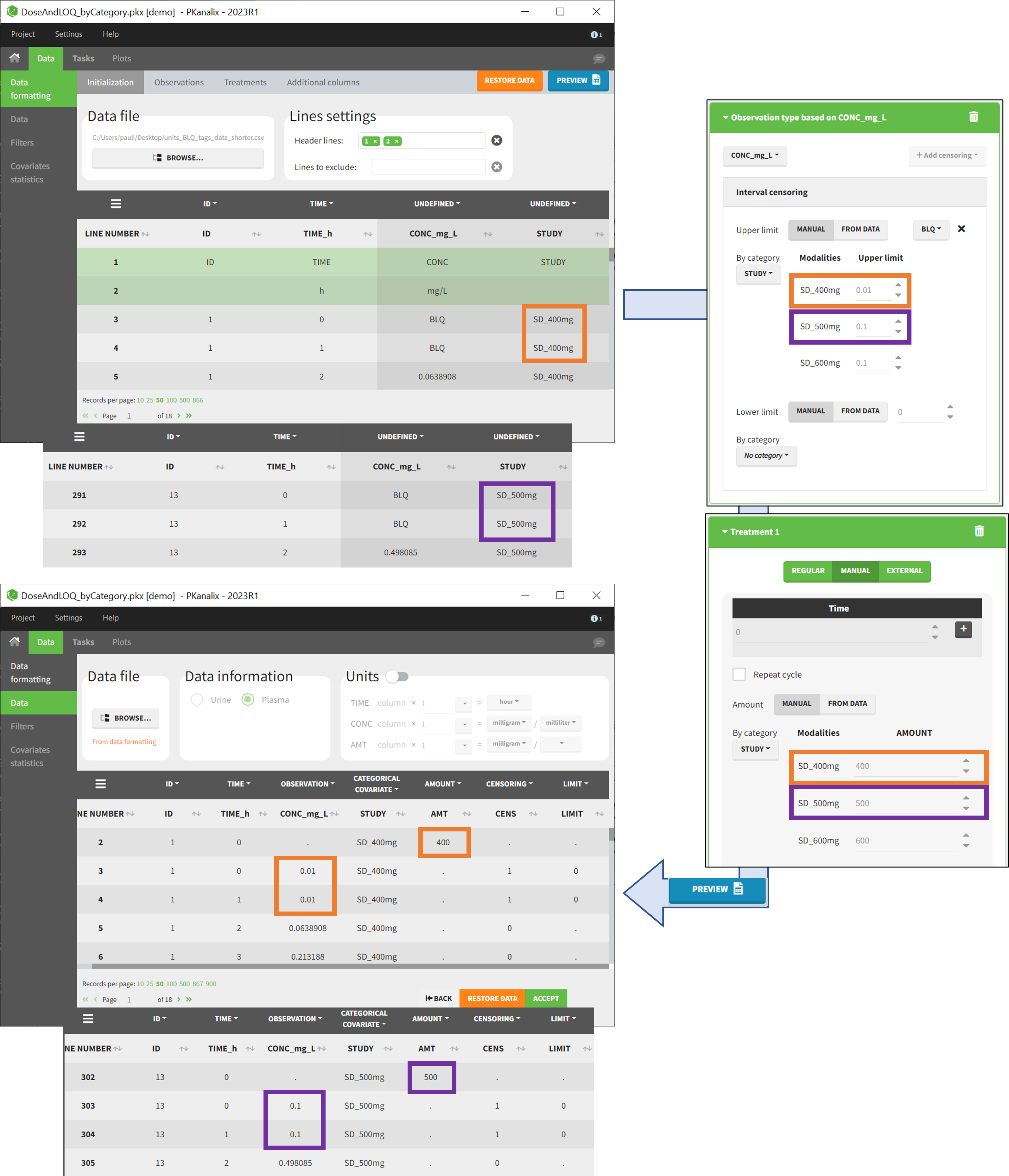
- demo DoseAndLOQ_byCategory.pkx (the screenshot below focuses on the formatting of doses and excludes other elements present in the demo):
In this demo there are three studies distinguished in the STUDY column with the categories “SD_400mg”, “SD_500mg” and “SD_600mg”. In Data Formatting, a single dose is manually defined at time 0 for all individuals, with different amounts depending the STUDY category. In addition, censoring interval is defined for the censoring tags BLQ, with an upper limit of the censoring interval (lower limit of quantification) that also depends on the STUDY category. Three new columns – AMT for dose amounts, CENS for censoring tags (0 or 1), and LIMIT for the lower limit of the censoring intervals – are created by Data Formatting. A new dose line is then inserted at time 0 for each individual.
From data
The option “From data” is used to directly read censoring limits, dose amounts, administration ids, infusion durations, or rates from a dataset’s column. The column must contain either numbers or numbers inside strings. In that case, the first number found in the string is extracted (including decimals with .).
- For censoring limits, the censoring limit used to replace each censoring tag is read from the selected column on the same row.
- For doses, the value chosen for the newly created column (AMT for amount, ADMID for administration id, INFDUR for infusion duration, INFRATE for infusion rate) on each new dose line is read from the selected column on the first row found in the dataset for the same individual and the same time as the dose, or the next time if there is no line in the initial dataset at that time, or the previous time if no time is found after the dose.
Example:
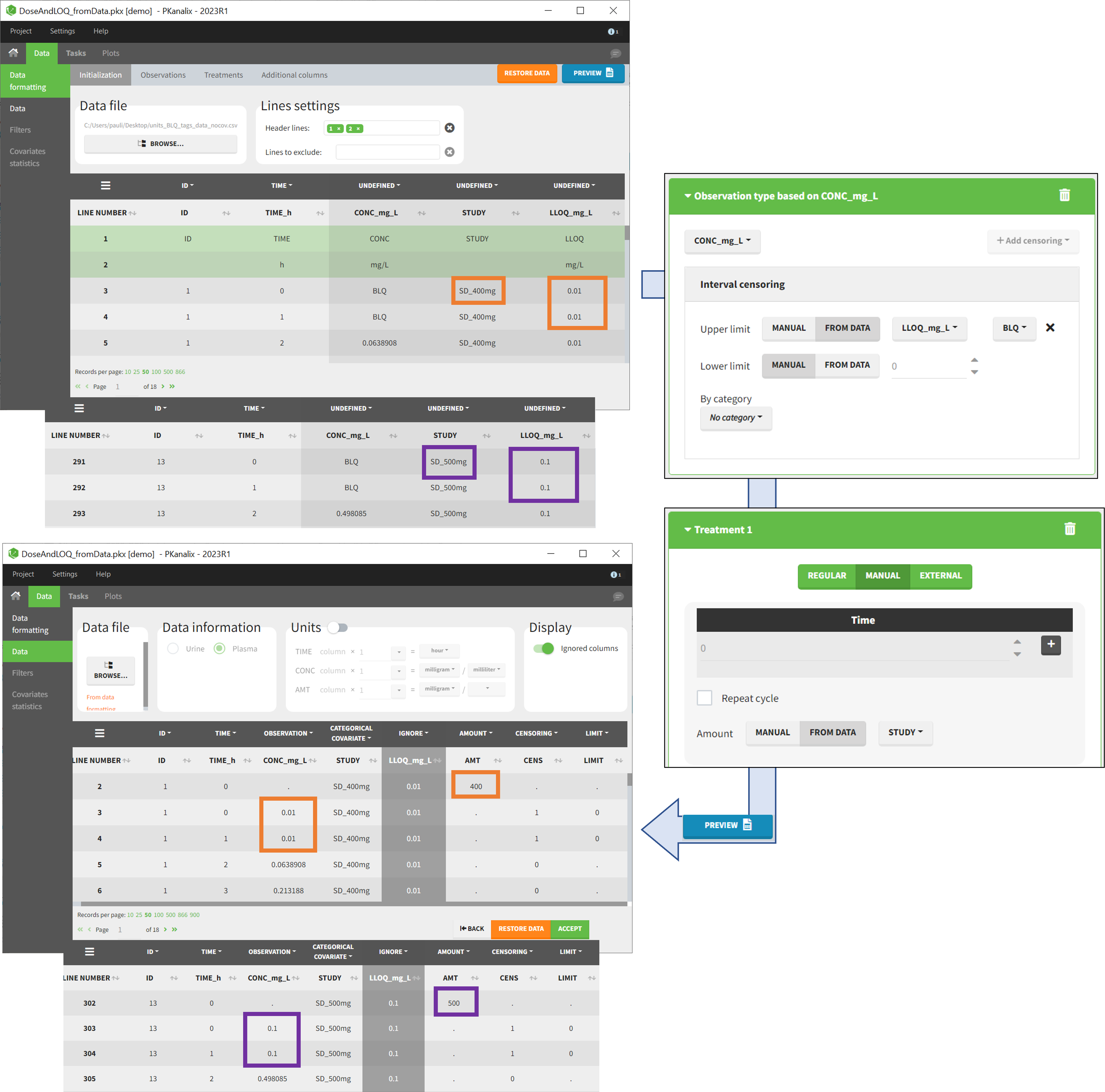
- demo DoseAndLOQ_fromData.pkx (the screenshot below focuses on the formatting of doses and censoring and excludes other elements present in the demo):
In this demo there are three studies distinguished in the STUDY column with the categories “SD_400mg”, “SD_500mg” and “SD_600mg”. In Data Formatting, a single dose is manually defined at time 0 for all individuals, with the amount read the STUDY column. In addition, censoring interval is defined for the censoring tags BLQ, with an upper limit of the censoring interval (lower limit of quantification) read from the LLOQ_mg_L column. Three new columns – AMT for dose amounts, CENS for censoring tags (0 or 1), and LIMIT for the lower limit of the censoring intervals – are created by Data Formatting. A new dose line is then inserted at time 0 for each individual, with amount 400, 500 or 600 for studies SD_400mg, SD_500mg and SD_600mg respectively.
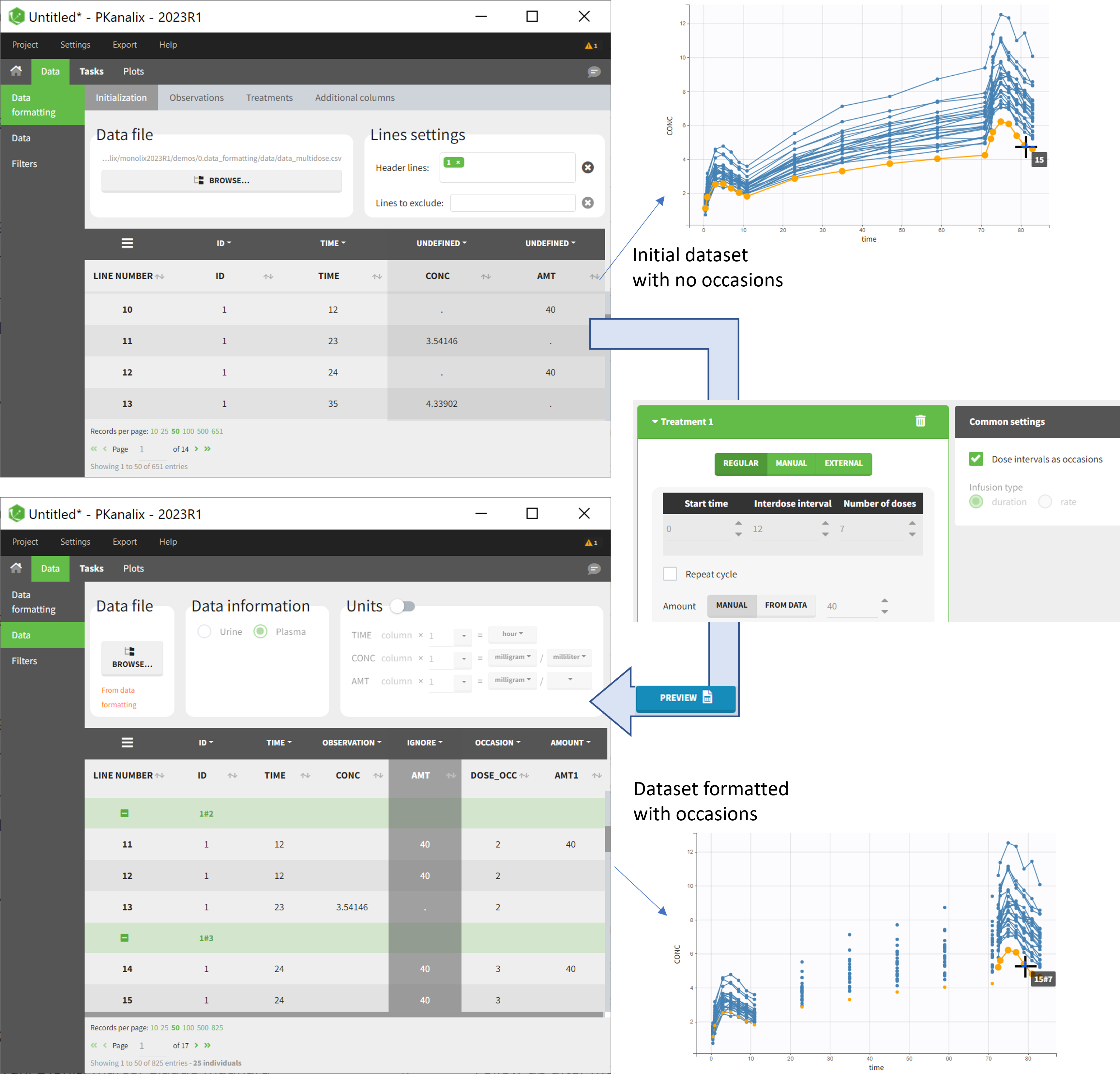
9. Creating occasions from dosing intervals
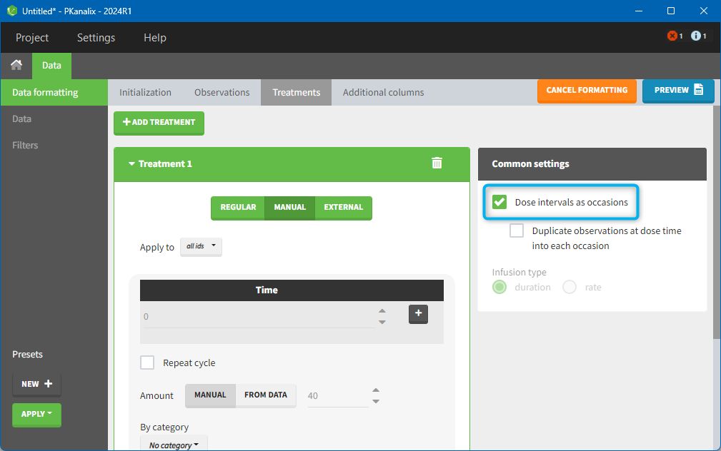
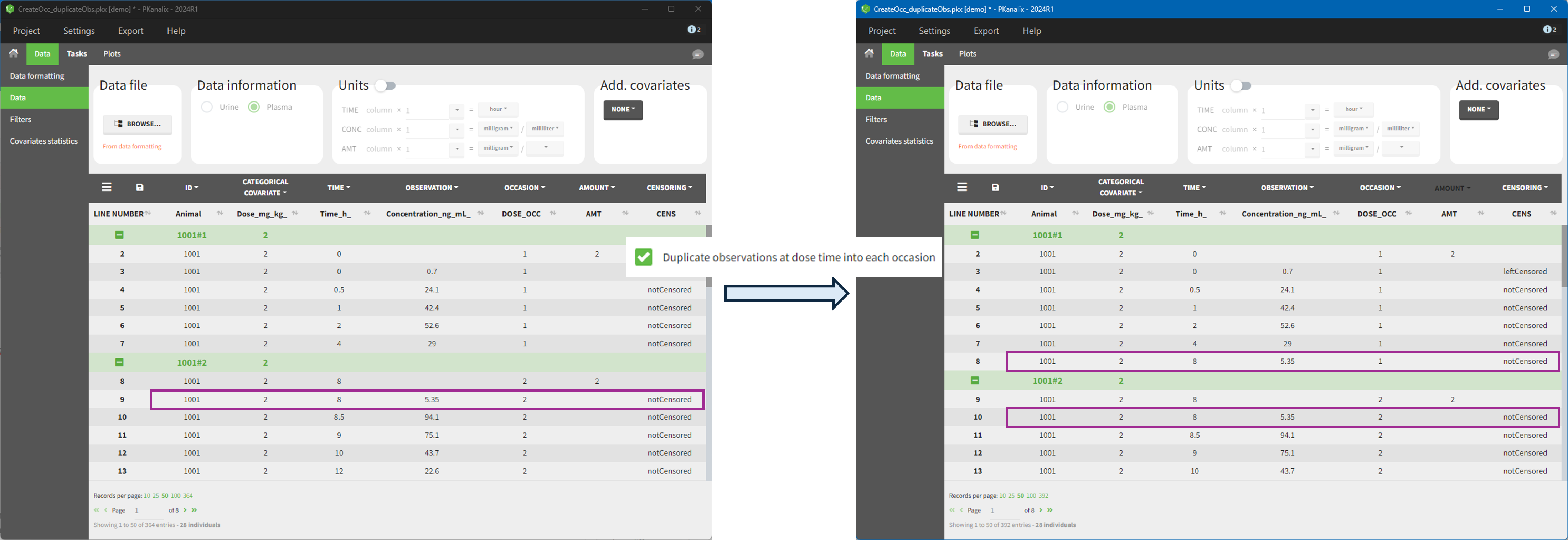
The option “Dose intervals as occasions” in the Treatments subtab of Data Formatting allows to create an occasion column to distinguish dose intervals. This is useful if the sets of measurements following different doses should be analyzed independently for a same individual. From the 2024 version on, an additional option “Duplicate observations at dose times into each occasion” is available. This option allows to duplicate the observations which are at exactly the same time as dose, such that they appear both as last point of the previous occasion and first point of the next occasion.
Example:
- demo doseIntervals_as_Occ.mlxtran (Monolix demo in the folder 0.data_formatting, here imported into PKanalix):
This demo imported from a Monolix demo has an initial dataset in Monolix-standard format, with multiple doses encoded as dose lines with dose amounts in the AMT column. When using this dataset directly into Monolix or PKanalix, a single analysis is done on each individual concentration profile considering all doses, which means that NCA would be done on the concentrations after the last dose only, and modeling (CA in PKanalix or population modeling in Monolix) would be estimated with a single set of parameter values for each individual. If instead we want to run separate analyses on the sets of concentrations following each dose, we need to distinguish them as occasions with a new column added with the Data Formatting module. To this end, we define the same treatment as in the initial dataset with Data Formatting (here as regular multiple doses) with the option “Dose intervals as occasions” selected. After clicking Preview, Data Formatting adds two new columns: an AMT1 column with the new doses, to be tagged as AMOUNT instead of the AMT column that will now be ignored, and a DOSE_OCC column to be tagged as OCCASION.
Example:
- demo CreateOcc_duplicateObs.pkx:

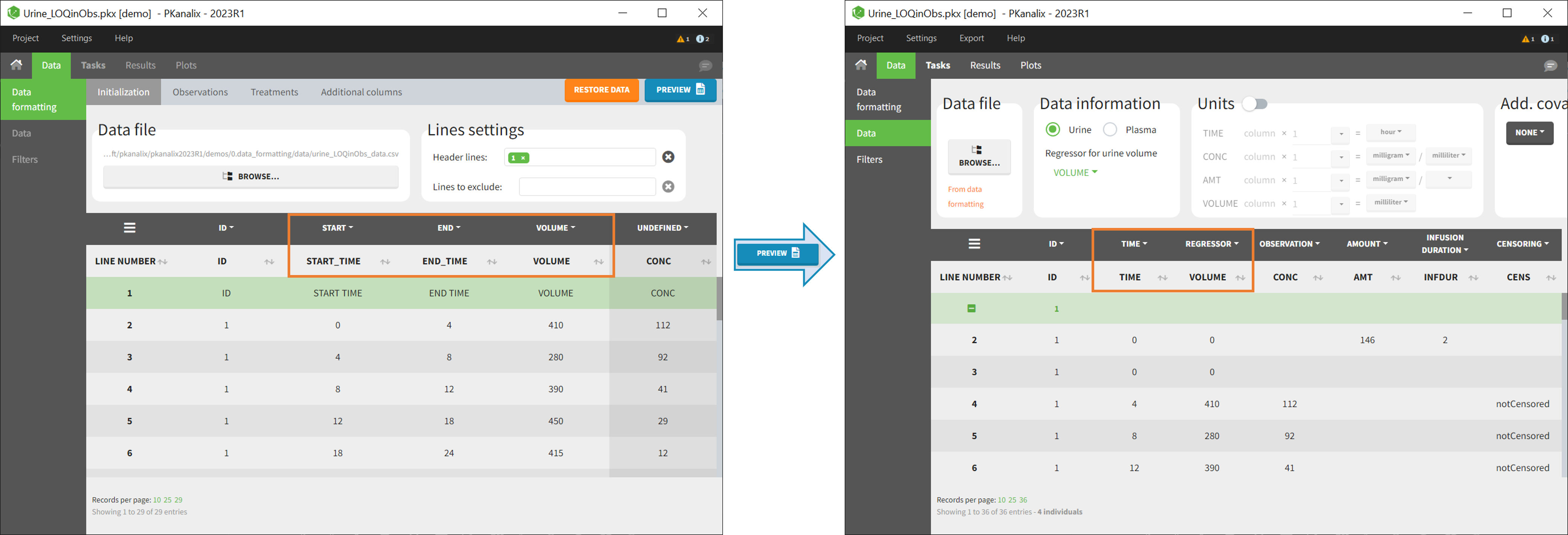
10. Handling urine data
In PKanalix-standard format, the start and end times of urine collection intervals must be recorded in a single column, tagged as TIME column-type, where the end time of an interval automatically acts as start time for the next interval (see here for more details). If a dataset contains start and end times in two different columns, they can be merged into a single column by Data Formatting. This is done automatically by tagging these two columns as START and END in the Initialization subtab of Data Formatting (see Section 2). In addition the column containing urine collection volume must be tagged as VOLUME.
Example:
- demo Urine_LOQinObs.plx:
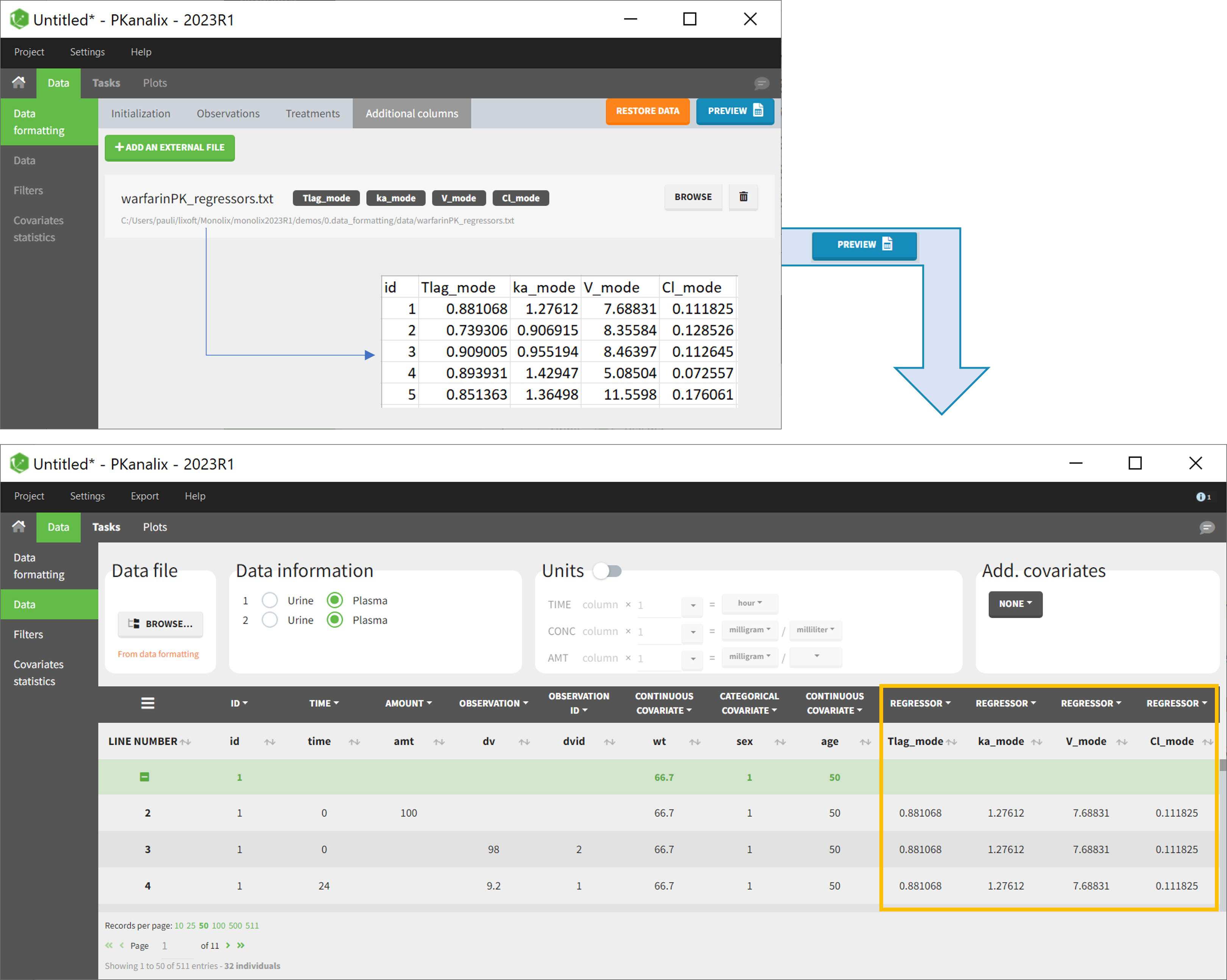
11. Adding new columns from an external file
The last subtab is used to insert additional columns in the dataset from a separate file. The external file must contain a table with a column named ID or id with the same subject identifiers as in the dataset to format, and other columns with a header name and individual values (numbers or strings). There can be only one value per individual, which means that the additional columns inserted in the formatted dataset can contain only a constant value within each individual, and not time-varying values.
Examples of additional columns that can be added with this option are:
- individual parameters estimated in a previous analysis, to be read as regressors to avoid estimating them. Time-varying regressors are not handled.
- new covariates.
If occasions are defined in the formatted dataset, it is possible to have an occasion column in the external file and values defined per subject-occasion.
Example:
- demo warfarin_PKPDseq_project.mlxtran (Monolix demo in the folder 0.data_formatting, here imported into PKanalix):
This demo imported from a Monolix demo has an initial PKPD dataset in Monolix-standard format. The option “Additional columns” is used to add the PK parameters estimated on the PK part of the data in another Monolix project.
12. Exporting the formatted dataset
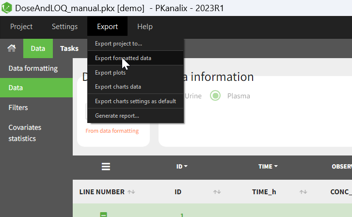
Once data formatting is done and the new dataset is accepted, the project can be saved and it is possible to export the formatted dataset as a csv file from the main menu Export > Export formatted data.
2.3.1.Data formatting presets
Starting from the 2024R1 version, if users need to perform the same or similar data formatting steps with each new project, a data formatting preset can be created and applied for new projects.
A typical workflow for using data formatting presets is as follows:
- Data formatting steps are performed on a specific project.
- Steps are saved in a data formatting preset.
- Preset is reapplied on multiple new projects (manually or automatically).
Creating a data formatting preset
After data formatting steps are done on a project, a preset can be created by clicking on the New button in the bottom left corner of the interface, while in the Data formatting tab:
Clicking on this button will open a pop-up window with a form that contains four parts:
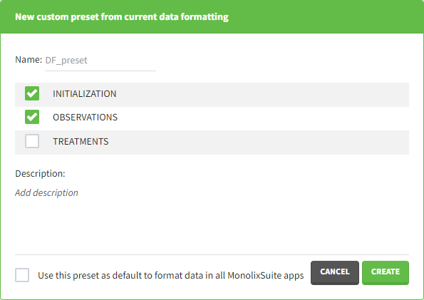
- Name: contains a name of the preset, this information will be used to distinguish between presets when applying them.
- Configuration: contains three checkboxes (initialization, observations, treatments). Users can choose which steps of data formatting will be saved in the preset. If option “External” was used in creating treatments, the external file paths will not be saved in the preset.
- Description: a custom description can be added.
- Use this preset as default to format data in all MonolixSuite apps: if ticked, the preset will be automatically applied every time a data set is loaded for data formatting in PKanalix and Monolix.
After saving the preset by clicking on Create, the description will be updated with the summary of all the steps performed in data formatting.
Important to note is that if a user wants to save censoring information in the data formatting preset, and the censored tags change between projects (e.g., censoring tag <LOQ=0.1> with varying numbers is used in different projects), the option “Use all automatically detected tags” should be used in the Observations tab. This way, no specific censoring tags will be saved in the preset, but they will be automatically detected and applied each time a preset is applied.
Applying a preset
A preset can be applied manually using the Apply button in the bottom left corner of the data formatting tab. Clicking on the Apply button will open a dropdown selection of all saved presets and the desired preset can be chosen.
The Apply button is enabled only after the initialization step is performed (ID and TIME columns are selected and the button Next was clicked). This allows PKanalix to fall back to the initialized state, if the initialization step from a preset fails (e.g., if ID and TIME column header saved in the presets do not exist in the new data set).
After applying a preset, all data formatting steps saved in the preset will try to be applied. If it is not possible to apply certain steps (e.g., some censoring tags or column headers saved in a preset do not exist), the error message will appear.
Managing presets
Presets can be created, deleted, edited, imported and exported by clicking on Settings > Manage Presets > Data Formatting.
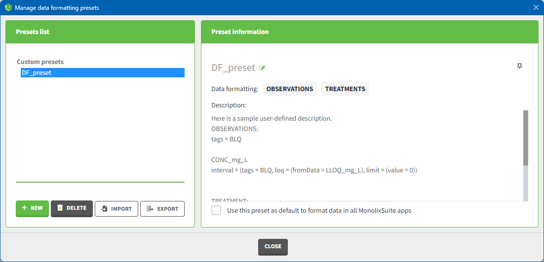
The pop-window allows users to:
- Create presets: clicking on the button New has the same behavior as clicking on the button New in the Data formatting tab (described in the section “Creating a data formatting preset”).
- Delete presets: clicking on the button Delete will permanently delete a preset. Clicking on this button will not ask for confirmation.
- Edit presets: by clicking on a preset in the left panel, the preset information will appear in the right panel. Name and preset description of the presets can then be updated, and a preset can be selected to automatically format data in PKanalix and Monolix.
- Export presets: a selected preset can be exported as a lixpst file which can be shared between users and imported using the Import button.
- Import presets: a user can import a preset from a lixpst file exported from another computer.
Additionally, an option to pin presets (always show them on top) can be used by clicking on the icon to facilitate the usage of presets when a user has a lot of them.
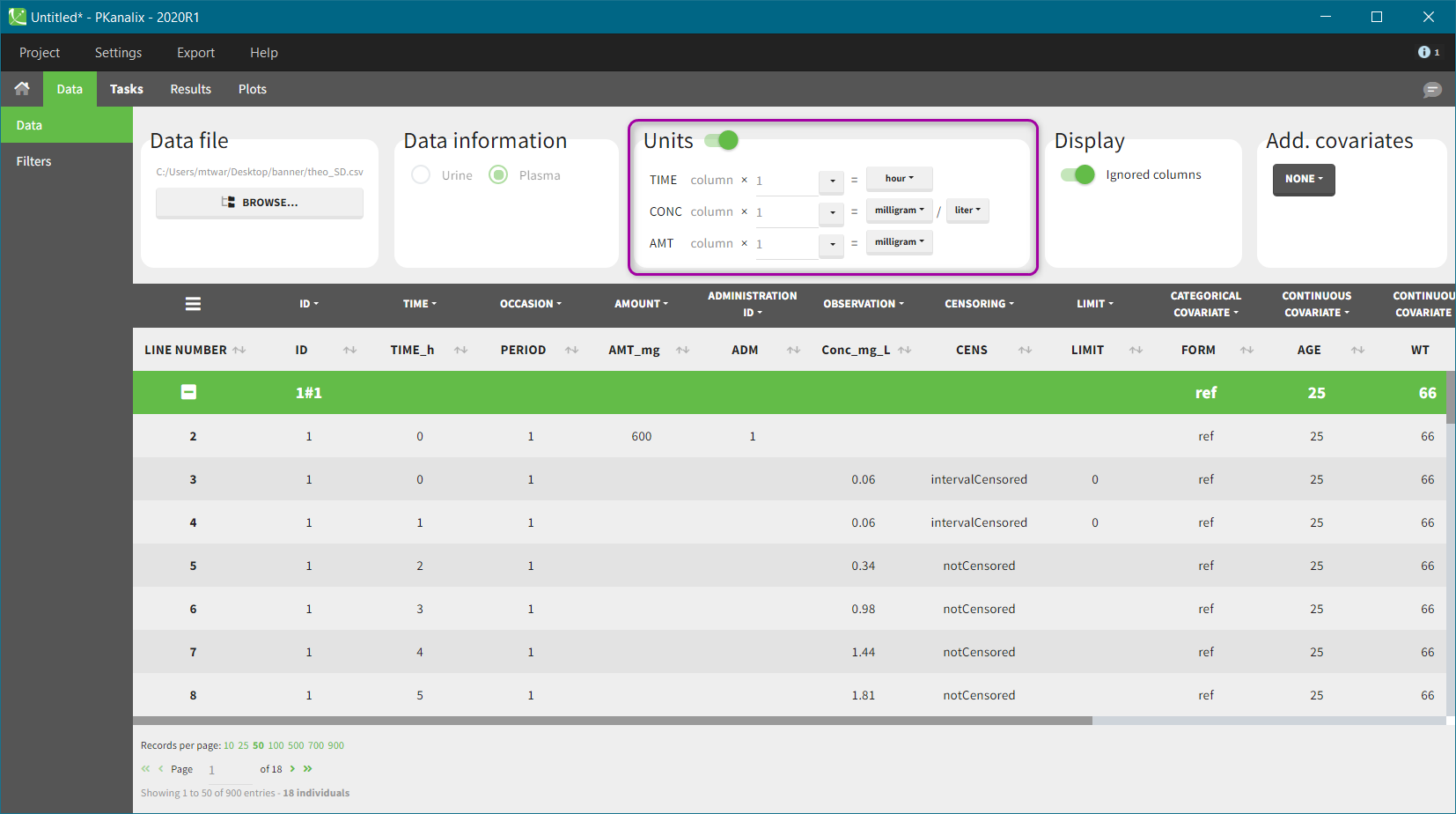
2.4.Units: display and scaling
- It displays units of the NCA and CA parameters calculated automatically from information provided by a user about units of measurements in a dataset. Units are shown in the results tables, on plots and are added to the saved files.
- It allows for scaling values of a dataset to represent outputs in preferred units, which facilitates the interpretation of the results. Scaling is done in the PKanalix data manager, and does not change the original data file.
- Units definition
- Units of the NCA parameters
- Units of the CA parameters
- Units display
- Units preferences
Units definition
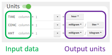
Units of the NCA and CA parameters are considered as combinations of units of: time, amount and volume. For instance, unit of AUC is [concentration unit * time unit] = [amount unit / volume unit * time unit]. These quantities correspond to columns in a typical PK dataset: time of measurements, observed concentration, dose amount (and volume of collected urine when relevant).
The “Units” block allows to define the preferred units for the output NCA parameters (purple frame below), which are related to the units of the data set columns (green frame below) via scaling factors (in the middle). The output units are displayed in results and plots after running the NCA and CA tasks.
In PKanalix version 2023R1, the amount can now also be specified in mass of the administered dose per body mass or body surface area. This eliminates the need to edit NCA or CA parameters by post-processing unit conversion.
Concentration is a quantity defined as “amount per volume”. It has two separate units, which are linked (and equal) to AMT and VOLUME respectively. Changing the amount unit of CONC will automatically update the amount unit of AMT. This constraint allows to apply simplifications to the output parameters units, for instance have Cmax_D as [mL] and not [mg/mL/mg].
Units without data conversion: Output units correspond to units of the input data.
In other words, desired units of the NCA and CA parameters correspond to units of measurements in the dataset. In this case, select from the drop-down menus units of the input data and keep the default scaling factor (equal to one). All calculations are performed using values in the original dataset and selected units are displayed in the results tables and on plots.
Units conversion: output units are different from the units of the input data.
NCA and CA parameters can be calculated and displayed in any units, not necessarily the same as used in the dataset. The scaling factors (by default equal to 1) multiply the corresponding columns in a dataset and transform them to a dataset in new units. PKanalix shows data with new, scaled values after having clicked on the “accept” button. This conversion occurs only internally and the original dataset file remains unchanged. So, in this case, select desired output units from the list and, knowing units of the input data, scale the original values to the new units.
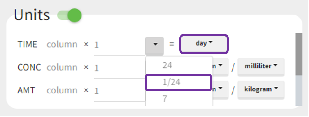
Example 1: input time units in [hours] and desired output units in [days]
For instance, let measurement times in a dataset be in hours. To obtain the outputs in days, set the output time unit as “days” and the scaling factor to 1/24, as shown below. It reads as follows:
(values of time in hours from the dataset) * (1/24) = time in days.
After accepting the scaling, a dataset shown in the Data tab is converted internally to a new data set. It contains original values multiplied by scaling factors. Then, all computations in the NCA and CA tasks are performed using new values, so that the results correspond to selected units.
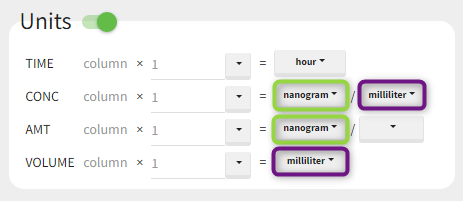
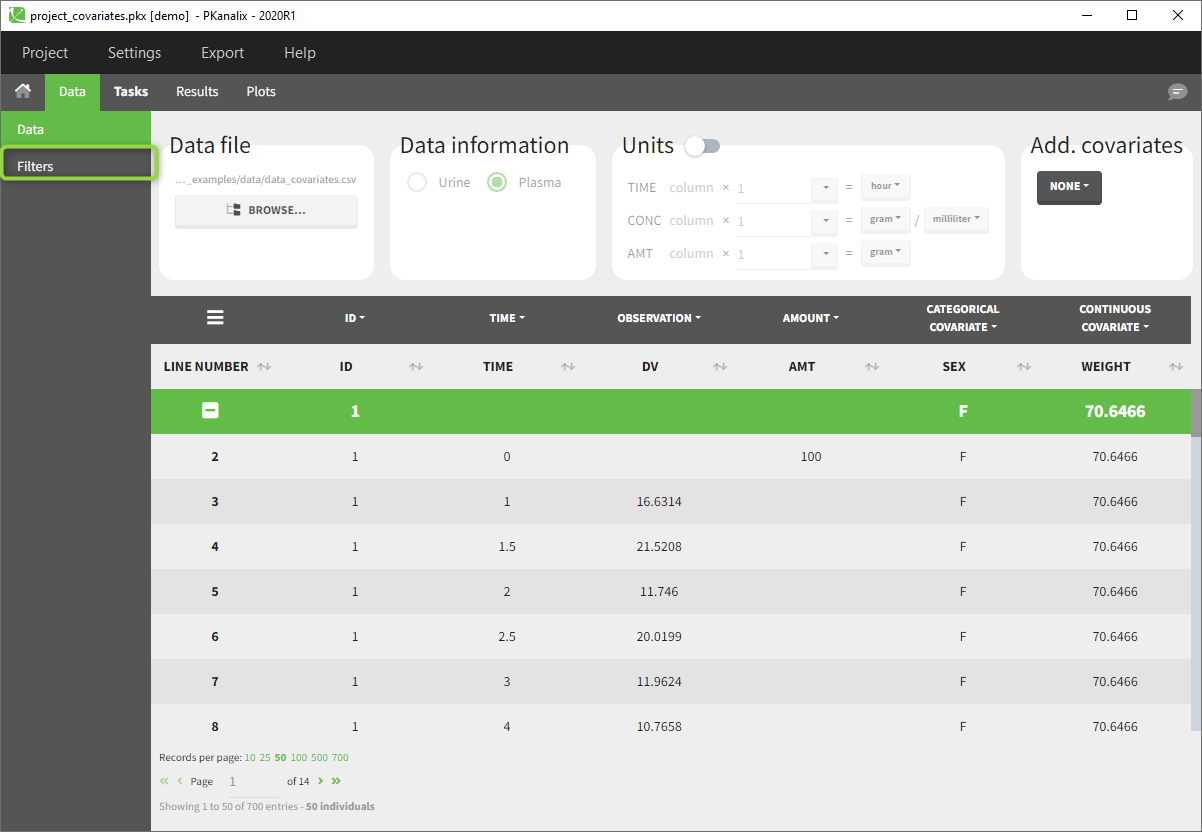
Example 2: input data set concentration units in [ng/mL] and amount in [mg]
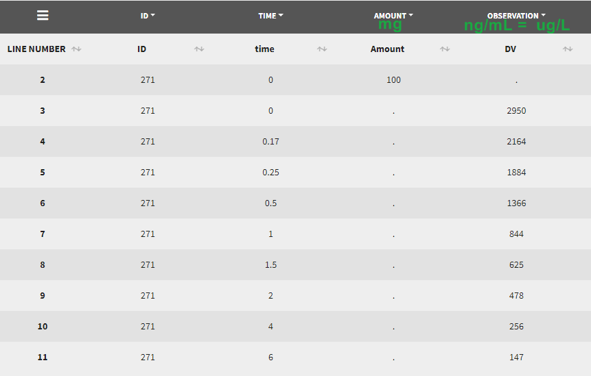 Let’s assume that we have a data set where the concentration units are [ng/mL]=[ug/L] and the dose amount units are [mg], as presented above. It is not possible to indicate these units directly, as the amount unit of CONC and AMT must be the same. One option would be to indicate the CONC as [mg/kL] and the AMT as [mg] but having the volume unit as [kL] is not very convenient. We will thus use the scaling factors to harmonize the units of the concentration and the amount.
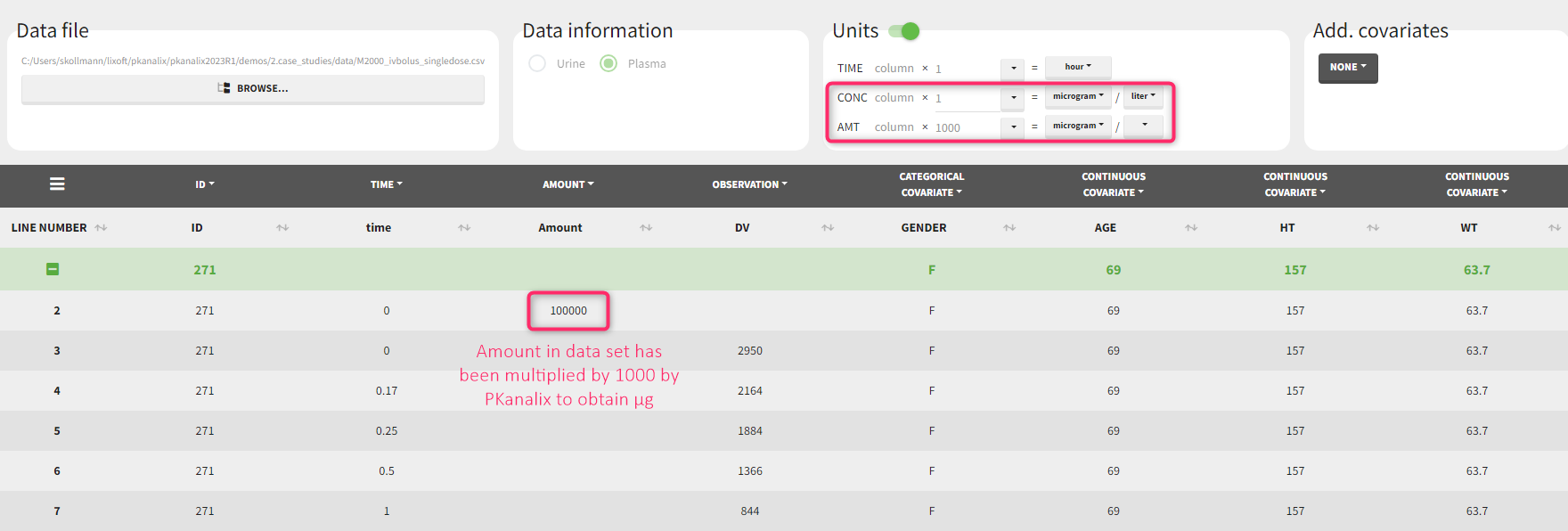
If we would like to have the output NCA parameters using [ug] and [L], we can define the CONC units as [µg/L] (as the data set input units) and scale the AMT to convert the amount column from [mg] to [ug] unit with a scaling factor of 1000. After clicking “accept” on the bottom right, the values in the amount column of the (internal) data set have been multiplied by 1000 by PKanalix such that they are now in [µg].
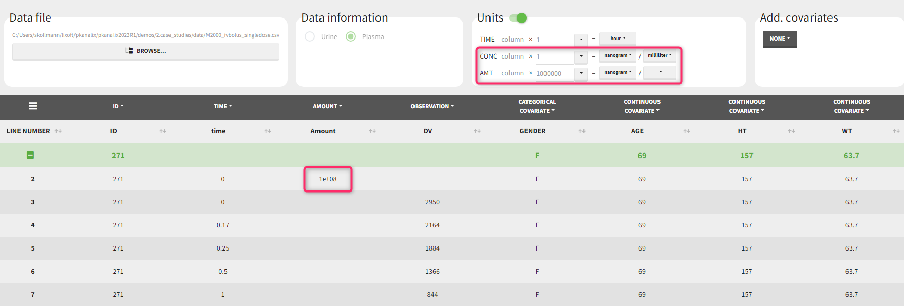
If we would like to have the output NCA parameters using [ng] and [mL], we can define the CONC units as [ng/mL] (as the data set input units) and scale the AMT to convert the amount column from [mg] to [ng] unit with a scaling factor of 1000000.
Units for the NCA parameters
| Rsq | no unit |
| Rsq_adjusted | no unit |
| Corr_XY | no unit |
| No_points_lambda_z | no unit |
| Lambda_z | time-1 |
| Lambda_z_lower | time |
| Lambda_z_upper | time |
| HL_lambda_z | time |
| Span | no unit |
| Lambda_z_intercept | no unit |
| T0 | time |
| Tlag | time |
| Tmax_Rate | time |
| Max_Rate | amount.time-1 |
| Mid_Pt_last | time |
| Rate_last | amount.time-1 |
| Rate_last_pred | amount.time-1 |
| AURC_last | amount |
| AURC_last_D | grading |
| Vol_UR | volume |
| Amount_recovered | amount |
| Percent_recovered | % [not calculable when grading -> set as NaN] |
| AURC_all | amount |
| AURC_INF_obs | amount |
| AURC_PerCentExtrap_obs | % |
| AURC_INF_pred | amount |
| AURC_PerCentExtrap_pred | % |
| C0 | amount.volume-1 |
| Tmin | time |
| Cmin | amount.volume-1 |
| Tmax | time |
| Cmax | amount.volume-1 |
| Cmax_D | grading.volume-1 |
| Tlast | time |
| Clast | amount.volume-1 |
| AUClast | time.amount.volume-1 |
| AUClast_D | grading.time.volume-1 |
| AUMClast | time2.amount.volume-1 |
| AUCall | time.amount.volume-1 |
| AUCINF_obs | time.amount.volume-1 |
| AUCINF_D_obs | grading.time.volume-1 |
| AUCINF_pred | time.amount.volume-1 |
| AUCINF_D_pred | grading.time.volume-1 |
| AUC_PerCentExtrap_obs | % |
| AUC_PerCentBack_Ext_obs | % |
| AUMCINF_obs | time2.amount.volume-1 |
| AUMC_PerCentExtrap_obs | % |
| Vz_F_obs | volume.grading-1 |
| Cl_F_obs | volume.time-1.grading-1 |
| Cl_obs | volume.time-1.grading-1 |
| Cl_pred | volume.time-1.grading-1 |
| Vss_obs | volume.grading-1 |
| Clast_pred | amount.volume-1 |
| AUC_PerCentExtrap_pred | % |
| AUC_PerCentBack_Ext_pred | % |
| AUMCINF_pred | time2.amount.volume-1 |
| AUMC_PerCentExtrap_pred | % |
| Vz_F_pred | volume.grading-1 |
| Cl_F_pred | volume.time-1.grading-1 |
| Vss_pred | volume.grading-1 |
| Tau | time |
| Ctau | amount.volume-1 |
| Ctrough | amount.volume-1 |
| AUC_TAU | time.amount.volume-1 |
| AUC_TAU_D | grading.time.volume-1 |
| AUC_TAU_PerCentExtrap | % |
| AUMC_TAU | time2.amount.volume-1 |
| Vz | volume.grading-1 |
| Vz_obs | volume.grading-1 |
| Vz_pred | volume.grading-1 |
| Vz_F | volume.grading-1 |
| CLss_F | volume.time-1.grading-1 |
| CLss | volume.time-1.grading-1 |
| CAvg | amount.volume-1 |
| FluctuationPerCent | % |
| FluctuationPerCent_Tau | % |
| Accumulation_index | no unit |
| Swing | no unit |
| Swing_Tau | no unit |
| Dose | amount.grading-1 |
| N_Samples | no unit |
| MRTlast | time |
| MRTINF_obs | time |
| MRTINF_pred | time |
| AUC_lower_upper | time.amount/volume |
| AUC_lower_upper_D | grading.time.volume-1 |
| CAVG_lower_upper | amount/volume |
| AURC_lower_upper | amount |
| AURC_lower_upper_D | grading |
Units for the PK parameters
Units are available only in PKanalix. When exporting a project to Monolix, values of PK parameters are re-converted to the original dataset unit. Below, volumeFactor is defined implicitly as: volumeFactor=amtFactor/concFacto, where “factor” is the scaling factor used in the “Units” block in the Data tab.
| PARAMETER | UNIT | INVERSE of UNITS |
| V (V1, V2, V3) | volume.grading-1 | value/volumeFactor |
| k (ka, k12, k21, k31, k13, Ktr) | 1/time | value*timeFactor |
| Cl, Q (Q2, Q3) | volume/time.grading-1 | value*timeFactor/volumeFactor |
| Vm | amount/time.grading-1 | value*timeFactor/amountFactor |
| Km | concentration | value/concFactor |
| T (Tk0, Tlag, Mtt) | time | value/timeFactor |
| alpha, beta, gamma | 1/time | value*timeFactor |
| A, B, C | grading/volume | value*volumeFactor |
Units display
To visualise units, switch on the “units toggle” and accept a dataset. Then, after running the NCA and CA tasks, units are displayed:
- In the results table next to the parameter name (violet frame), in the table copied with “copy” button
 (blue frame) and in the saved .txt files in the result folder (green frame).
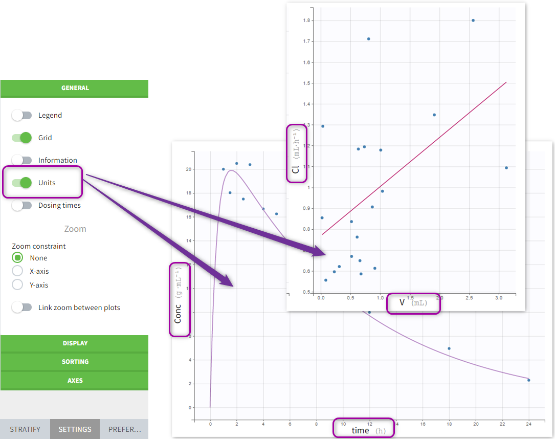
- On plots if the “units” display is switched on in the General plots settings
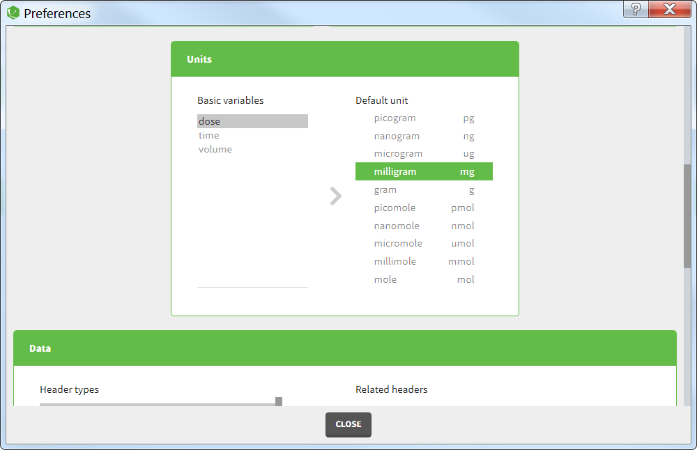
Units preferences
The units selected by default when starting a new PKnaalix project can be chosen in the menu Settings > Preferences.
2.5.Filtering a data set
Starting on the 2020 version, filtering a data set to only take a subpart into account in your modelization is possible. It allows to make filters on some specific IDs, times, measurement values,… It is also possible to define complementary filters and also filters of filters. It is accessible through the filters item on the data tab.
- Creation of a filter
- Filtering actions
- Filters with several actions
- Other filers: filter of filter and complementary filters
Creation of a filter
To create a filter, you need to click on the data set name. You can then create a “child”. It corresponds to a subpart of the data set where you will define your filtering actions.
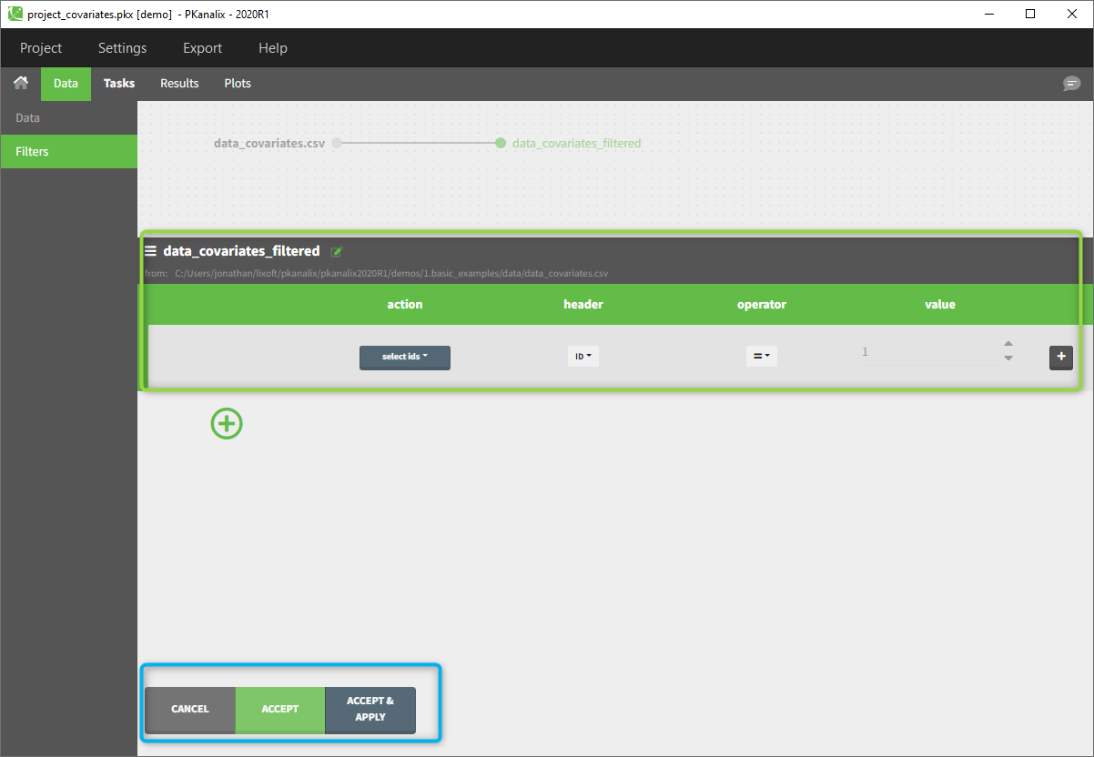
You can see on the top (in the green rectangle) the action that you will complete and you can CANCEL, ACCEPT, or ACCEPT & APPLY with the bottoms on the bottom.
Filtering a data set: actions
In all the filtering actions, you need to define
- An action: it corresponds to one of the following possibilities: select ids, remove ids, select lines, remove lines.
- A header: it corresponds to the column of the data set you wish to have an action on. Notice that it corresponds to a column of the data set that was tagged with a header.
- An operator: it corresponds to the operator of choice (=, ≠, < ≤, >, or ≥).
- A value. When the header contains numerical values, the user can define it. When the header contains strings, a list is proposed.
For example, you can
- Remove the ID 1 from your study:

In that case, all the IDs except ID = 1 will be used for the study. - Select all the lines where the time is less or equal 24:

In that case, all lines with time strictly greater that 24 will be removed. If a subject has no measurement anymore, it will be removed from the study. - Select all the ids where SEX equals F:
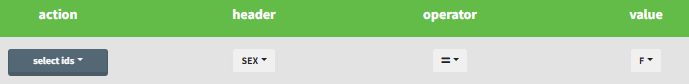
In that case, all the male will be removed of the study. - Remove all Ids where WEIGHT less or equal 65:
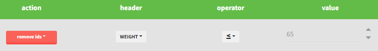
In that case, only the subjects with a weight over 65 will be kept for the study.
In any case, the interpreted filter data set will be displayed in the data tab.
Filters with several actions
In the previous examples, we only did one action. It is also possible to do several actions to define a filter. We have the possibility to define UNION and/or INTERSECTION of actions.
INTERSECTION
By clicking by the + and – button on the right, you can define an intersection of actions. For example, by clicking on the +, you can define a filter corresponding to intersection of
- The IDs that are different to 1.
- The lines with the time values less than 24.

Thus in that case, all the lines with a time less than 24 and corresponding to an ID different than 1 will be used in the study. If we look at the following data set as an example
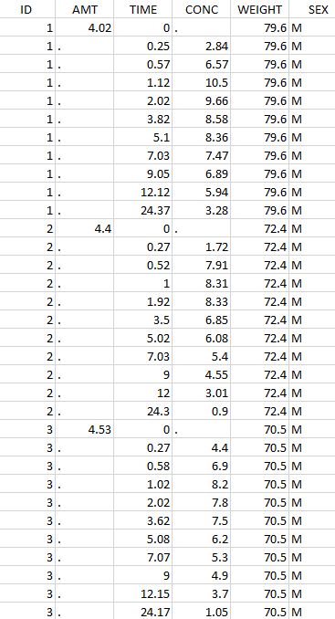 Initial data set |
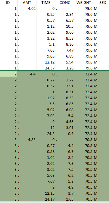 Resulting data set after action: select IDs ≠ 1 Resulting data set after action: select IDs ≠ 1 |
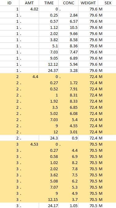 Considered data set for the study as the intersection of the two actions |
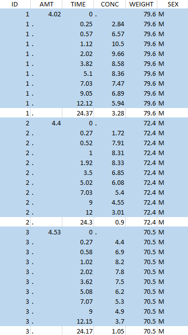 Resulting data set after action: select lines with time ≤ 24 Resulting data set after action: select lines with time ≤ 24 |
UNION
By clicking by the + and – button on the bottom, you can define an union of actions. For example, in a data set with a multi dose, I can focus on the first and the last dose. Thus, by clicking on the +, you can define a filter corresponding to union of
- The lines where the time is strictly less than 12.
- The lines where the time is greater than 72.
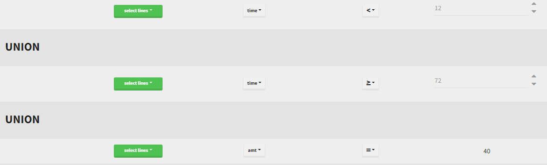
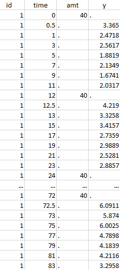 Initial data set |
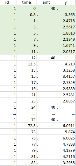 Resulting data set after action: select lines where the time is strictly less than 12 |
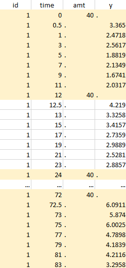 Considered data set for the study as the union of the three actions |
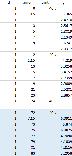 Resulting data set after action: select lines where the time is greater than 72 |
||
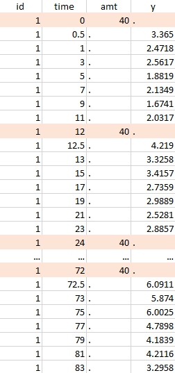 Resulting data set after action: select lines where amt equals 40 |
Notice that, if just define the first two actions, all the dose lines at a time in ]12, 72[ will also be removed. Thus, to keep having all the doses, we need to add the condition of selecting the lines where the dose is defined.
In addition, it is possible to do any combination of INTERSECTION and UNION.
Other filers: filter of filter and complementary filters
Filtering a data set can be nested. Based on the definition of a filter, by clicking on the filter, it is possible to create:
- A child: it corresponds to a new filter with the initial filter as the source data set.
- A complement: corresponds to the complement of the filter. For example, if you defined a filter with only the IDs where the SEX is F, then the complement corresponds to the IDs where the SEX is not F.
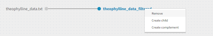
2.6.Import a Monolix/Simulx project
MonolixSuite applications are interconnected and projects can be exported/imported between different applications. This interconnection is guaranteed by using the same model syntax (mlxtran language) and the same dataset format.
There are two options to create a PKanalix project from a Monolix or Simulx project*
- Import a Monolix project to PKanalix to run NCA or CA on the original dataset in the Monolix project
- Export from Monolix to PKanalix to run NCA or CA on the original dataset, or on the VPC simulations or individual fits
- Export from Simulx to PKanalix to run NCA or CA on simulations
*Note: Import and export to PKanalix is available starting from the 2023 version. In the previous versions, you can only export a PKanalix project to Monolix.
Import a Monolix project to PKanalix
To import a Monolix project, open PKanalix application and in the home page select IMPORT FROM:
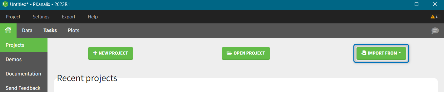
In PKanalix, it is possible to import only a Monolix project with its original dataset. When you select in the home screen IMPORT FROM > Monolix, then PKanalix will create a new, untitled, project with:
- Dataset tagging and formatting steps if present as in the Monolix project.
- Dataset filters if applied as in the Monolix project.
- NCA settings: “administration type” set to intravenous or extravascular depending on the administration in a model selected in the Monolix project.
- NCA settings: “observation ID to use” set to the first one alphabetically (if obsid are strings) or numerically (if obsid are integers).
- NCA settings: default PKanalix settings for the integral method, treatment of BLQ values, parameters.
- Acceptance criteria: not selected.
- Bioequivalence: default PKanalix settings
- CA model: set to the same structural model and the same mapping between observation ids and model outputs as in the Monolix project
- CA initial parameter values: equal to the initial estimates of the Monolix project
- CA parameters constraints: none for normally distributed parameters, positive for log-normally distributed parameters; bounded with limits imported from the Monolix project for logit-normally and probit-normally distributed parameters.
- CA calculations settings: default PKanalix settings
After the import, you can save the PKanalix project as usual, edit it and run the analysis.
Remark: Importing a Monolix project to PKanalix is only with the original dataset used to create a Monolix project. Export from Monolix to PKanalix has more options. You can choose to import a Monolix project with its original dataset, vpc dataset or with individual fits dataset, see the next section. Import from Simulx is currently unavailable.
Export from Monolix to PKanalix
To export a Monolix project to PKanalix click EXPORT PROJECT TO in the top menu “Export”:
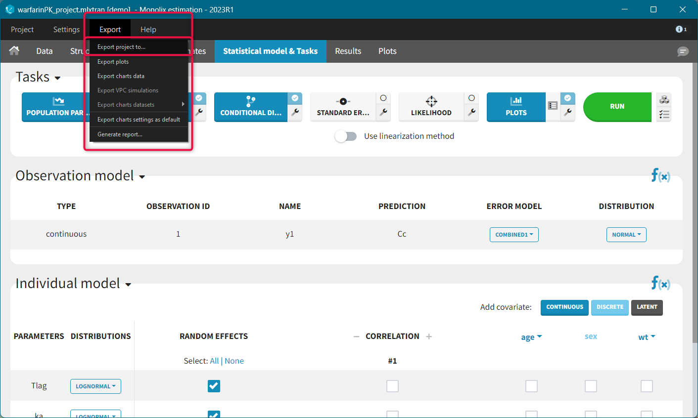
When you export a Monolix project, in the export pop-up window you can choose:
- to which application you want to export your current project: PKanalix or Simulx: select “PKanalix”
- which dataset you want to use in the export: original dataset, vpc dataset, individual fits dataset
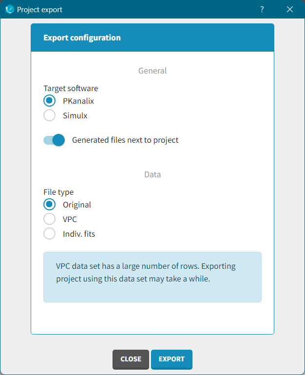
By default, Monolix will copy all files, e.g. dataset and model, next to the new PKanalix project. To keep current location of these files, switch the toggle “Generated files next to project” off. Click the “EXPORT” button at the bottom to confirm. PKanalix application will open automatically with a predefined project called “untitled”. It will contain the same pre-defined elements as during the import, see the description above. If you selected export with vpc dataset or individual fits dataset, then Monolix creates a .csv files with vpc simulations or individual model predictions in the MonolixSuite data format. These dataset will be automatically loaded in the new PKanalix project.
Export with individual fits dataset
The .csv generated file contains model predictions on a fine time grid (specified in the Plots tasks settings in Monolix) obtained with different individual parameters:
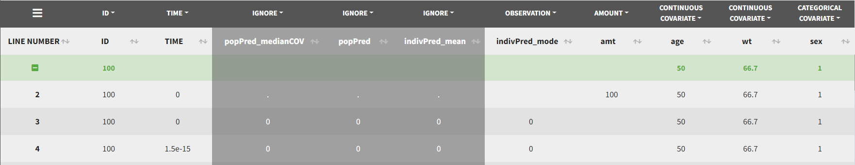
- popPred: model predictions with individual parameters corresponding to the population parameters estimated by Monolix and the impact of the individual covariates, but random effects set to zero. For instance,\( V_i = V_{pop} \times exp^{\beta_{V,WT}\times WT_i} \)
- popPred_medianCOV: model predictions with individual parameters corresponding to the population parameters and the impact of the covariates using the population median for continuous covariates and reference category for categorical covariates, and random effects set to zero. For instance, \( V_i = V_{pop} \times exp^{\beta_{V,WT}\times WT_{med}} \)
- indivPred_mode: [when EBEs task has run] model predictions with individual parameters corresponding to the EBEs (conditional mode) estimated by Monolix (as displayed in Monolix Results > Indiv. param > Cond. mode.). Tagged as OBSERVATION by default.
- indivPred_mean: [when COND. DISTRIB. task has run] model predictions with individual parameters corresponding to the conditional mean estimated by Monolix (as displayed in in Monolix Results > Indiv. param > Cond. mean.)
The dataset contains also the individual design: doses, occasions, regressors, covariates.
Export with vpc dataset
The .csv generated dataset in the Monolix format constructed from the VPC simulations and individual design (doses, occasions, regressors, covariates)
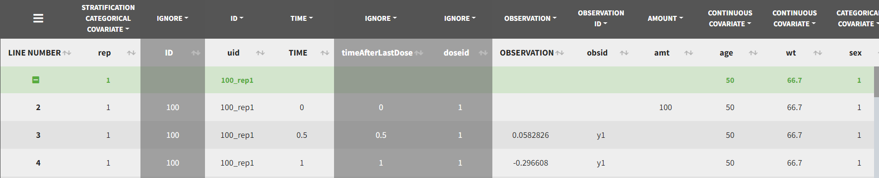
- rep: simulation replicate. Tagged as stratification categorical covariate
- uid: unique id obtained by concatenation of “rep” and “id”. Tagged as ID by default.
- time/timeAfterLastDose: observation times or times after last dose
- doseid: administration id
- y1/observation: simulated observation values. Default header is “y1” if a model has only one output, and “observation” in case of several outputs (obsid column is created automatically). Tagged automatically as OBSERVATION
3.Non Compartmental Analysis
One of the main feature of PKanalix is the calculation of the parameters in the Non Compartmental Analysis framework.
NCA task
Main function of PKanalix is to calculate PK metrics (non-compartmental parameters). In the Tasks tab, you find a dedicated section “NCA” (left panel). There are two subtabs: RUN and CHECK \(\lambda_z\).
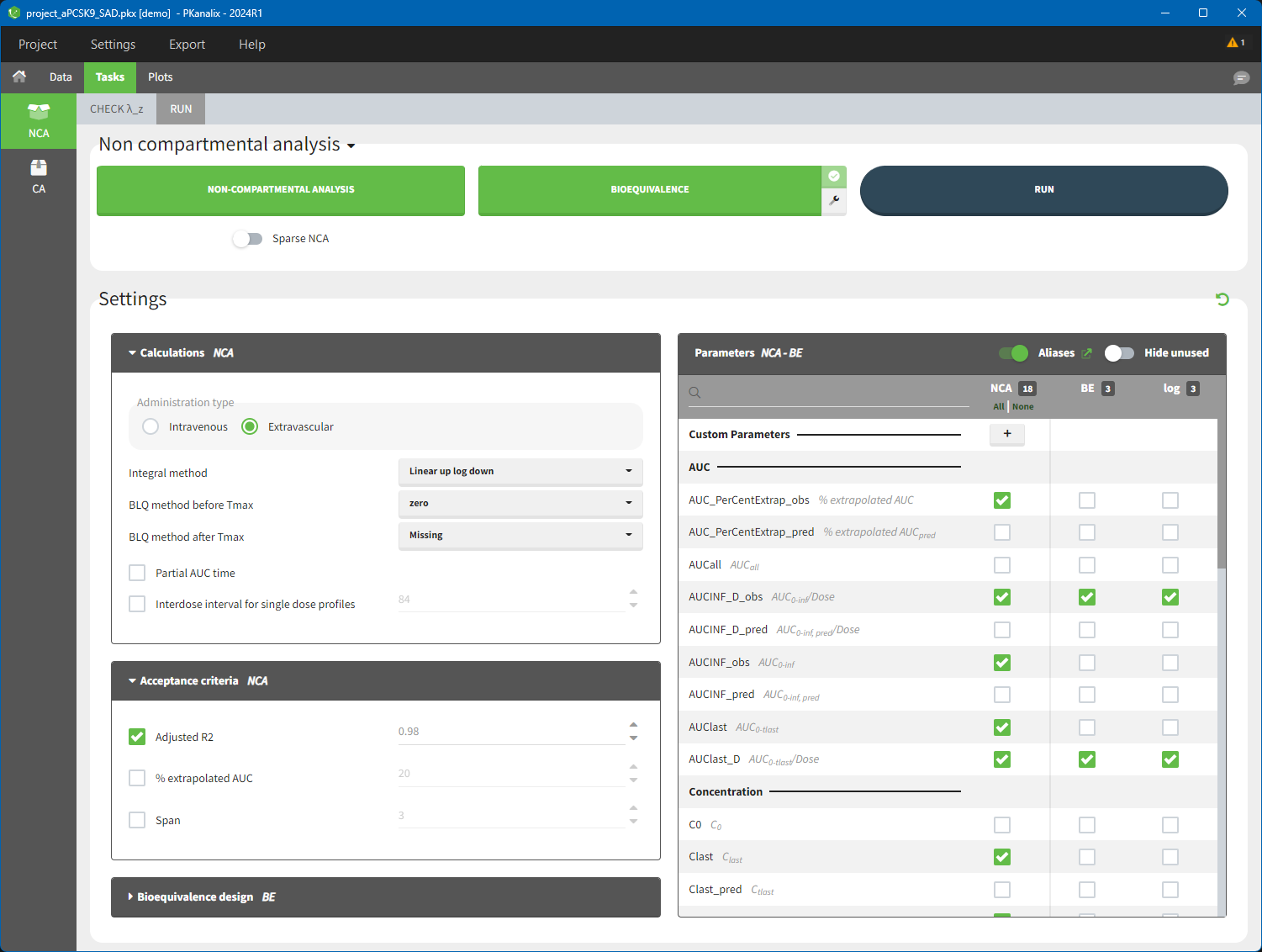
- RUN tab contains section with calculation task buttons (for non-compartmental analysis and bioequivalence) and the settings: calculation, acceptance criteria, parameters and bioequivalence design. The meaning of all the settings and their default is in a separate page here.
- CHECK \(\lambda_z\) allows to define the calculation of \(\lambda_z\) – it is a graphical preview of each individual data and the regression line, more details are here.
To calculate NCA parameters click on the button NON-COMPARTMENTAL ANALYSIS. If you click on RUN button, then PKanalix runs all selected tasks (“in green”). Results and plots are automatically generated in separate tabs.
NCA results
When you run the NCA task, results are automatically generated and displayed in the RESULTS tab. There are three tables: individual estimates, summary and points for λ_z.
Non compartmental analysis results per individual
Individual estimates of the NCA parameters are displayed in the table in the tab “INDIV. ESTIM.”
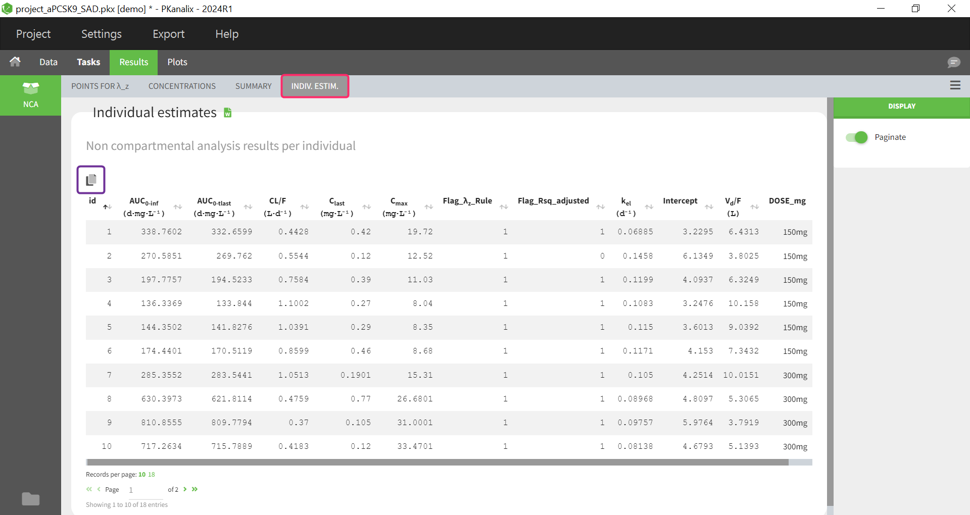
All the computed parameters depend on the type of observation and administration. Description of all the parameters is here. You can copy this table to a word or an excel file using an icon on the top right (purple frame).
In addition to generated flag variables defined by defined acceptance criteria in the NCA settings here, the Flag_\( \lambda_{z}\)_Rule column is now available since version 2024. If the inclusion/exclusion of data points in the calculation of lambda z do not follows the main rule (data points have been manually selected), the Flag_\( \lambda_{z}\)_Rule column is filled with 0, otherwise with 1.
Summary statistics on NCA results
Statistics on non-compartmental parameters are displayed in the summary table in the sub-tab “SUMMARY”. Description of all the summary calculation is here.
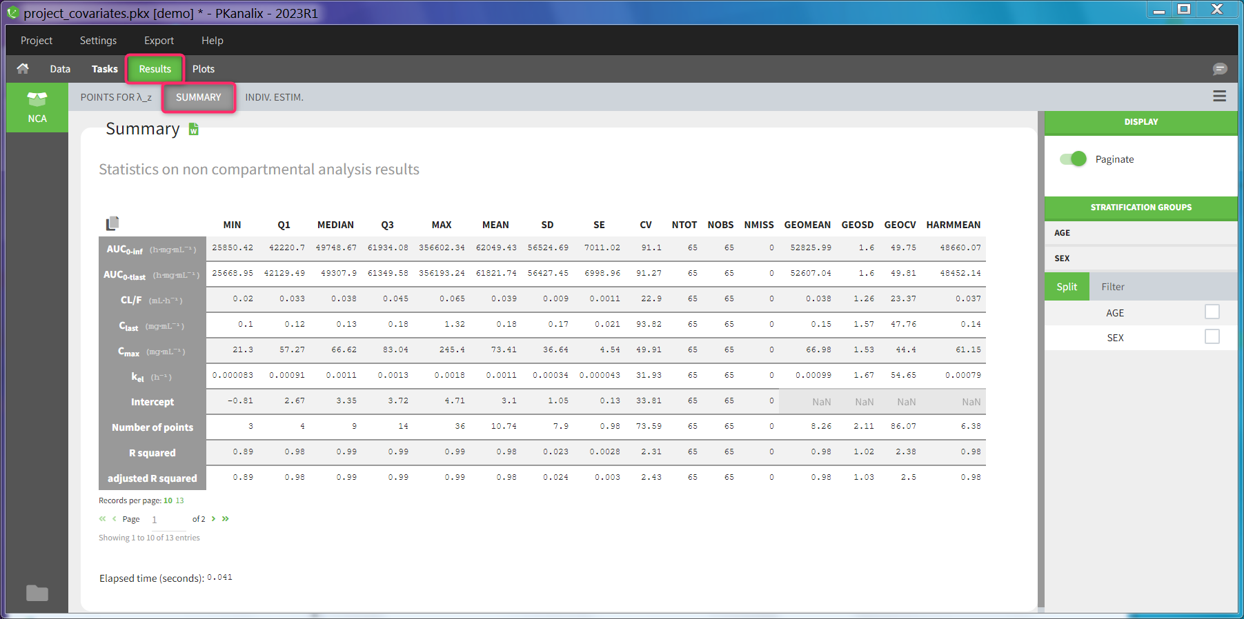
The summary table can be
- split and filtered according to the categorical and continuous covariates tagged in the data set
- filtered according to the acceptance criteria defined in the NCA settings
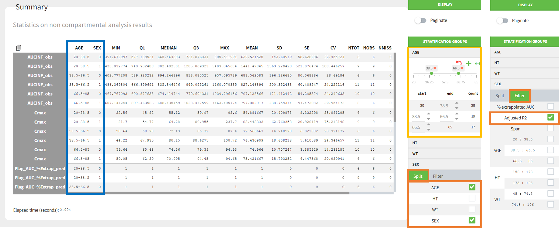
- Split by covariates: When you apply “split” of a table, the values of the splitting covariates are displayed in the first columns of the summary table (blue highlight). The order of these columns corresponds to the order of the clicks to setup the splitting covariates (orange highlight). You can discretized continuous covariates into groups by defining the group limits (yellow highlight), and create new categories for categorical covariates (drug and drop to merge existing categories).
It is currently not possible to split the table in several subtables (instead of splitting the rows), nor to choose the orientation of the table (NCA parameters as columns for instance). See the reporting documentation for details how these options can be applied in a report. - Filter by acceptance criteria: you can remove from the calculations in the summary table parameter values from subjects that do not meet the acceptance criteria
Read details on filtering rules
- When filtering by the “% extrapolated AUC” criterion, values from subjects that do not meet the criterion are excluded for the following parameters: [AUCINF_obs, AUCINF_pred, AUCINF_D_obs, AUCINF_D_pred, AUC_PerCentExtrap_obs, AUC_PerCentExtrap_pred, Vz_obs, Vz_pred, Vz_F_obs, Vz_F_pred, Cl_obs, Cl_pred, Cl_F_obs, Cl_F_pred, AUMCINF_obs, AUMCINF_pred, AUMC_PerCentExtrap_obs, AUMC_PerCentExtrap_pred, MRTINF_obs, MRTINF_pred, Vss_obs, Vss_pred, AURC_INF_obs, AURC_INF_pred, AURC_PerCentExtrap_obs, AURC_PerCentExtrap_pred].
- When filtering by the “Adjusted R2” or “Span” criteria, all parameters in the previous list are similarly impacted, as well as the additional following parameters: [Rsq, Rsq_adjusted, Corr_XY, Lambda_z, Lambda_z_intercept, Lambda_z_lower, Lambda_z_upper, HL_Lambda_z, Span, Clast_pred, No_points_lambda_z, AUC_PerCentBack_Ext_obs, AUC_PerCentBack_Ext_pred, Rate_last_pred].
- The following parameters are not impacted by the filtering: [AUC_T1_T2 AUC_T1_T2_D, AUC_TAU, AUC_TAU_D, AUC_TAU_PerCentExtrap, AUCall, AUClast, AUClast_D, AUMC_TAU, Accumulation_Index, C0, CLss, Cavg, Cavg_0_20, Clast, Cmax, Cmax_D, Cmin, Ctau, Ctrough, Dose, FluctuationPerCent, FluctuationPerCent_Tau, N_Samples, Swing, Swing_Tau, T0, Tau, Tlast, Tmax, Tmin, Vz]. In particular, parameters that relate to steady-state or partial AUC are not filtered, even though they rely on the lambda_z value for extrapolation when no valid observation is available at the upper end of the interval.
When you save a PKanalix project, the stratification settings of the results are saved in the result folder and are reloaded when reloading a PKanalix project. The table in the <result folder>/PKanalix/IndividualParameters/nca/ncaIndividualParametersSummary.txt takes into account the split definition. This table is generated when clicking “run” in the task tab (usually without splits, as the result tab is not yet available to define them) and also upon saving the project (with splits if defined).
Table of concentrations
With MonolixSuite version 2024, a table of concentrations is now generated after each NCA. It can either be displayed as a summary table or as a table for individual concentrations.
Summary table of concentrations
This table is displayed by default. The columns contain the concentrations of different time points, which are summarised along the rows by different descriptive metrics.

If nominal time is available in the dataset, the concentrations are automatically summarized using nominal time points. By disabling the toggle in the right panel, the table can also be displayed based on the actual time contained in the dataset.
The same stratification and filter options are available as for the NCA summary table.
The rules established in the NCA task tab for handling censored data are also considered in the calculation of the descriptive statistics.
Table of individual concentrations
This table can be displayed in the same tab by enabling the toggle “Display individual profiles” in the right-hand side panel.
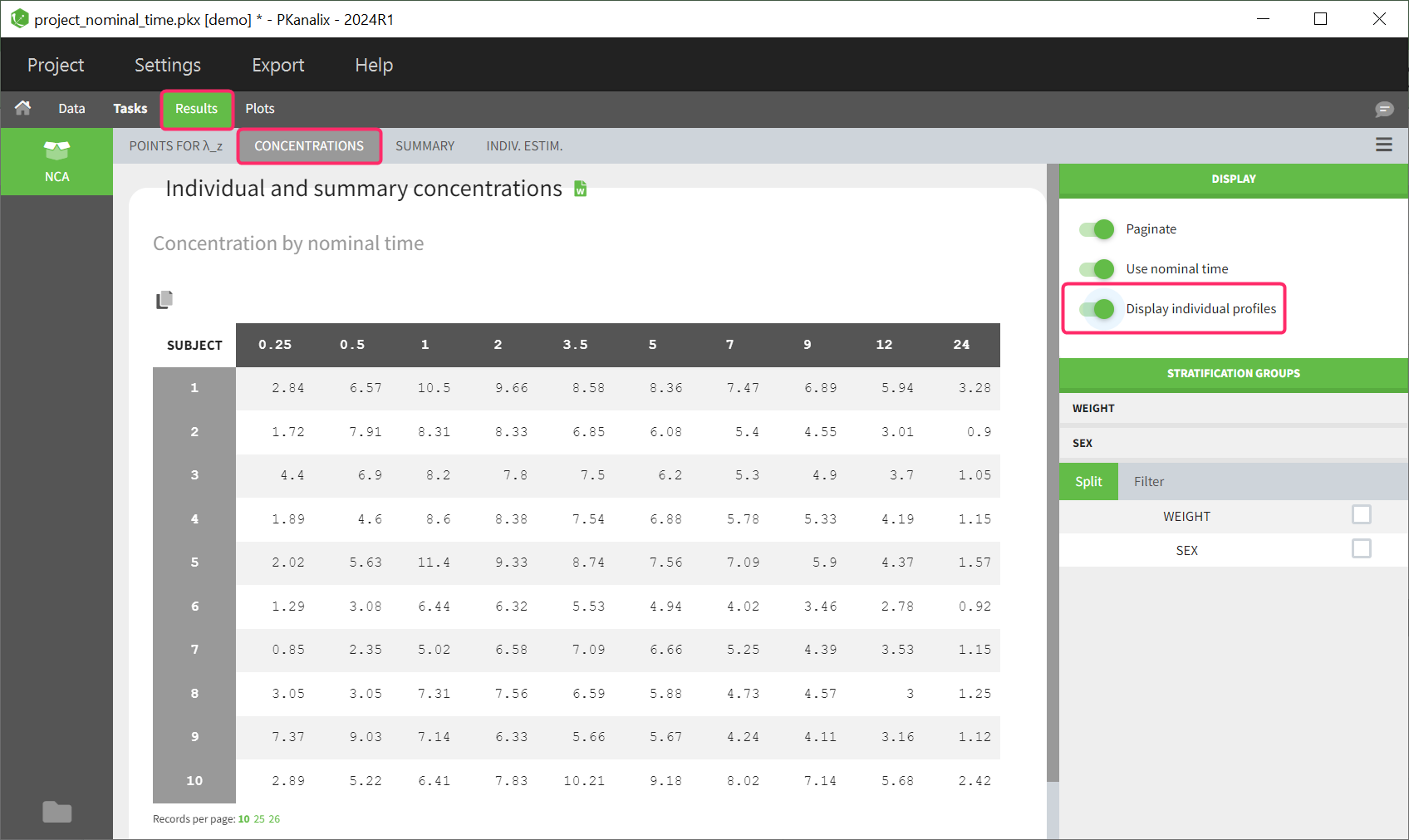 Each row in the table corresponds to an individual. The columns correspond to the different time points. There are options for stratification and filtering. Additionally, displaying the columns based on the nominal time or actual time points is also optional. Extrapolated points at dosing time are not displayed in the table as well as unused data for NCA, such as datapoints before last dose or negative values.
If the dataset contains left censored data, these will be displayed in the individual table of concentrations using the “<LLOQ” tag.
Ratios for NCA parameters
With MonolixSuite version 2024, parameter ratios can be calculated if required. Once this task has been performed, the results are displayed in 2 different tables in the results tab, as a summary table and as a table of individual ratios.
Summary table of ratios
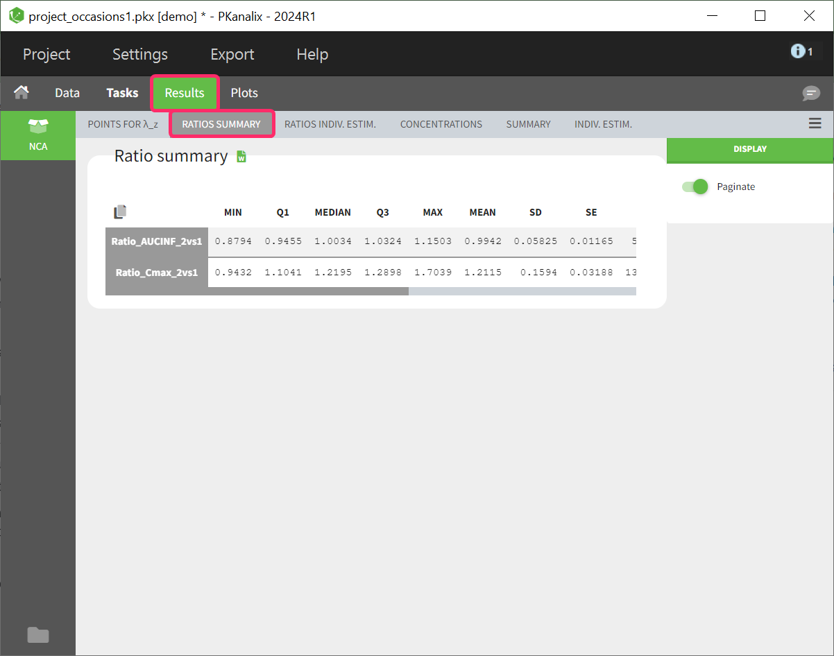
The calculated parameter ratios are presented using basic descriptive statistics. However, even if the dataset contains additional covariates or occasions, this table cannot be further stratified.
Table of ratios per individual
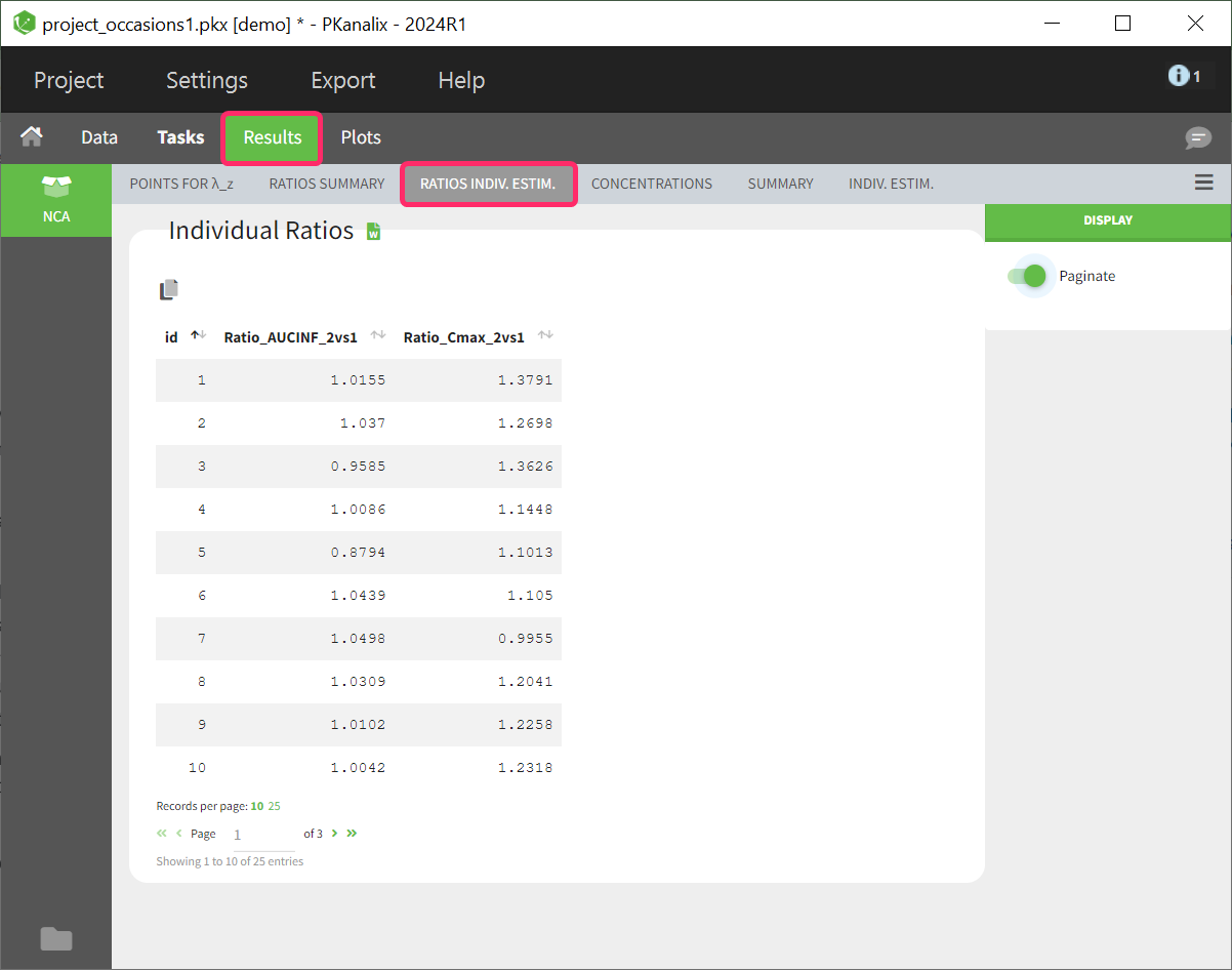
The parameter ratio is calculated per individual. This table shows a list sorted by subject identifier. The number of columns in the table depends on how many ratios have been defined. If a ratio couldn’t be calculated for a subject, such as due to missing values, NaN is displayed as the entry for the corresponding ratio parameter.
Points for lambda_z
In the sub-tab “POINTS FOR λ_z ” you find table of concentration points used for the terminal slope (λz) calculation.
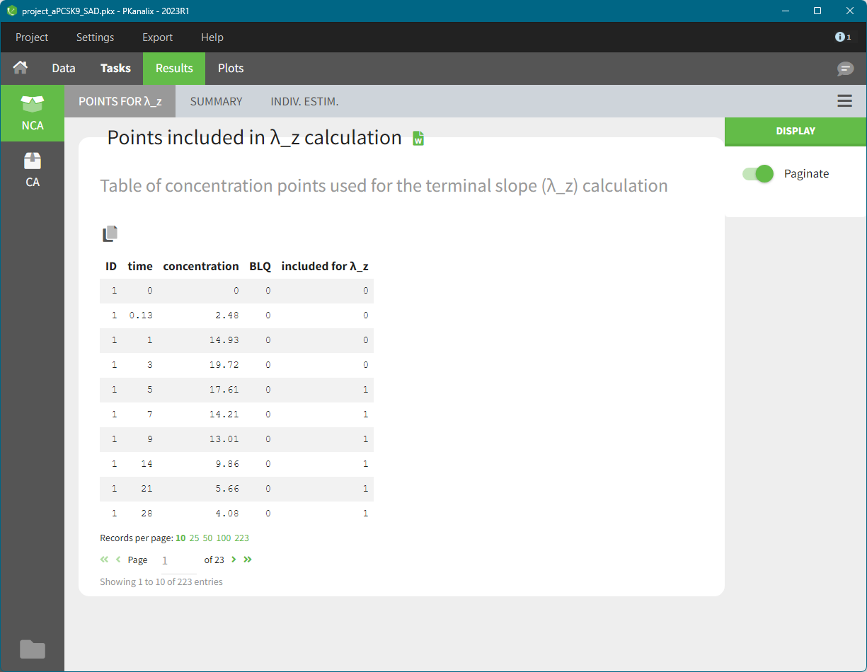
This table is displayed only if number of rows <5000. Above this, the tab appears as usual but with incomplete data. You can find the full table in the result folder: <result folder>/PKanalix/IndividualParameters/nca/pointsIncludedForLambdaZ.txt.
NCA plots
The PLOTS tab shows plot associated to the individual parameters:
- Correlation between NCA parameters: displays scatter plots for each pair of parameters. It allows to identify correlations between parameters, which can be used to see the results of your analysis and see the coherence of the parameters for each individuals.
- Distribution of the NCA parameters: shows the empirical distribution of the parameters. it allows to verify distribution of parameters over the individuals.
- NCA parameters w.r.t. covariates: displays the individual parameters as a function of the covariates. It allows to identify correlation effects between the individual parameters and the covariates.
- NCA individual fits: shows the lambdaZ regression line for each individual.
- NCA data: displays the data according to the NCA settings as spaghetti plot
NCA outputs
After running the NCA task, the following files are available in the result folder: <resultFolder>/PKanalix/IndividualParameters/nca
- Summary.txt contains the summary of the NCA parameters calculation, in a format easily readable by a human (but not easy to parse for a computer)
- ncaIndividualParametersSummary.txt contains the summary of the NCA parameters in a computer-friendly format.
- The first column corresponds to the name of the parameters
- The second column corresponds to the CDISC name of the parameters
- The other columns correspond to the several elements describing the summary of the parameters (as explained here)
- ncaIndividualParameters.txt contains the NCA parameters for each subject-occasion along with the covariates.
- The first line corresponds to the name of the parameters
- The second line corresponds to the CDISC name of the parameters
- The other lines correspond to the value of the parameters
- pointsIncludedForLambdaZ.txt contains for each individual the concentration points used for the lambda_z calculation.
- id: individual identifiers
- occ: occasions (if present). The column header corresponds the data set header of the column(s) tagged as occasion(s).
- time: time of the measurements
- concentration: concentration measurements as displayed in the NCA individual fits plot (i.e after taking into the BLQ rules)
- BLQ: if the data point is a BLQ (1) or not (0)
- includedForLambdaZ: if this data point has been used to calculate the lambdaZ (1) or not (0)
The files ncaIndividualParametersSummary.txt and ncaIndividualParameters.txt can be exported in R for example using the following command
read.table("/path/to/file.txt", sep = ",", header = T)
Remarks
- To load the individual parameters using PKanalix name as headers, your just need to skip the second line
ncaParameters = read.table("/path/to/file.txt", sep = ",", header = T); ncaParameters[-1,] # to remove the CDISC name line - To load the individual parameters using CDISC as headers, your just need to skip the second line
ncaParameters = read.table("/path/to/file.txt", sep = ",", header = T, skip = 1) - The separator is the one defined in the user preferences. We set “,” in this example as it is the one by default.
3.1.Check lambda_z
The \(\lambda_z\) is the slope of the terminal elimination phase. If estimated, the NCA parameters will be extrapolated to infinity. Check lambda_z tab visualizes the linear regression model for each individual and allows to control the points included in the calculation of the \(\lambda_z\) parameter.
General rule
The “Check lambda_z” tab shows the data of each individual plotted by default on y-axis log-scale.
- Points used in the \(\lambda_z\) calculation are in blue.
- Points not used in the \(\lambda_z\) calculation are in grey.
- The \(\lambda_z\) curve is in green.
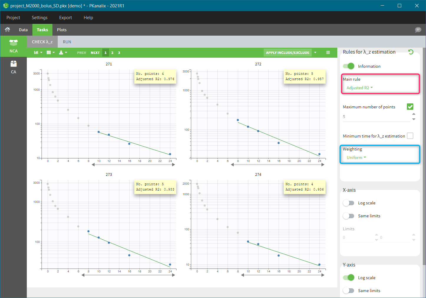
A main rule to select which points to include in the \(\lambda_z\) calculation applies to all individuals. You find it on top in the right panel – red frame in the figure above. There are four methods in a drop-down menu:
- “R2” chooses the number of points that optimize the correlation coefficient.
- “Adjusted R2” (called “Best Fit” in Winonlin) optimizes the adjusted correlation coefficient, taking into account the number of points. The “maximum number of points” and “minimum time” allow to further restrict the points selection.
- “Interval” selects all points within a given time interval.
- “Points” corresponds to the number of terminal points taken into account in the calculation.
The calculation of the \(\lambda_z\) is via the linear regression. The selection of the weighting used in the cost function is in the right panel (blue highlight). Three options are available: uniform (default), 1/Y, 1/Y^2.
See the Settings page and the Calculations page for more details. In addition to the main rule, it is possible to define more precisely (manually) which points to include or exclude for each individual.
Manual choice of measurements for the \(\lambda_z\) calculation
Charts in the check lambda_z tab are interactive. For each individual specific points can be selected manually to be included or excluded from the \(\lambda_z\) calculation. There are two methods to do it: define a range (time interval) with a slider or select each point individually.
Change of the range
For a given individual, the grey arrow below each individual chart defines a range – time interval when measured concentrations are used in the lambda-z calculation. New points to include are colored in light blue, and points to remove are colored in dark grey, as in the following figure:
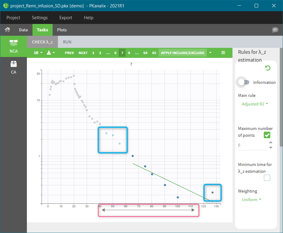
The button APPLY INCLUDE/EXCLUDE in the top – right corner of the chart area applies the manual modifications of the points in the calculation of the \(\lambda_z\). If modifications concern several individuals, then clicking on the “Apply include/exclude” button updates all of them automatically.
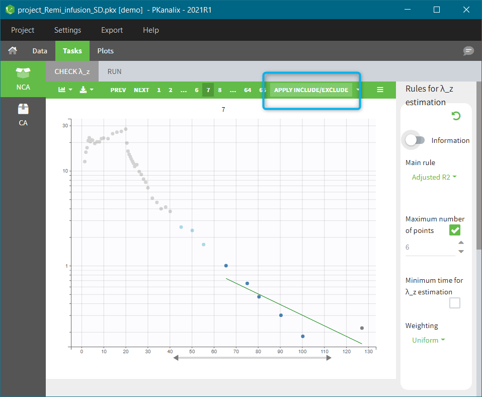
The plots are updated with new points and new \(\lambda_z\) curve. For modified plots, the “return arrow” appears in the top – left corner, red frame in the figure below. It resets the individual calculation to the general rule. The drop-down menu in the “Apply include/exclude” (blue frame) allows to reset all individuals to the general rule. Clear selection the current selection made before clicking on the “Apply include/exclude” button.
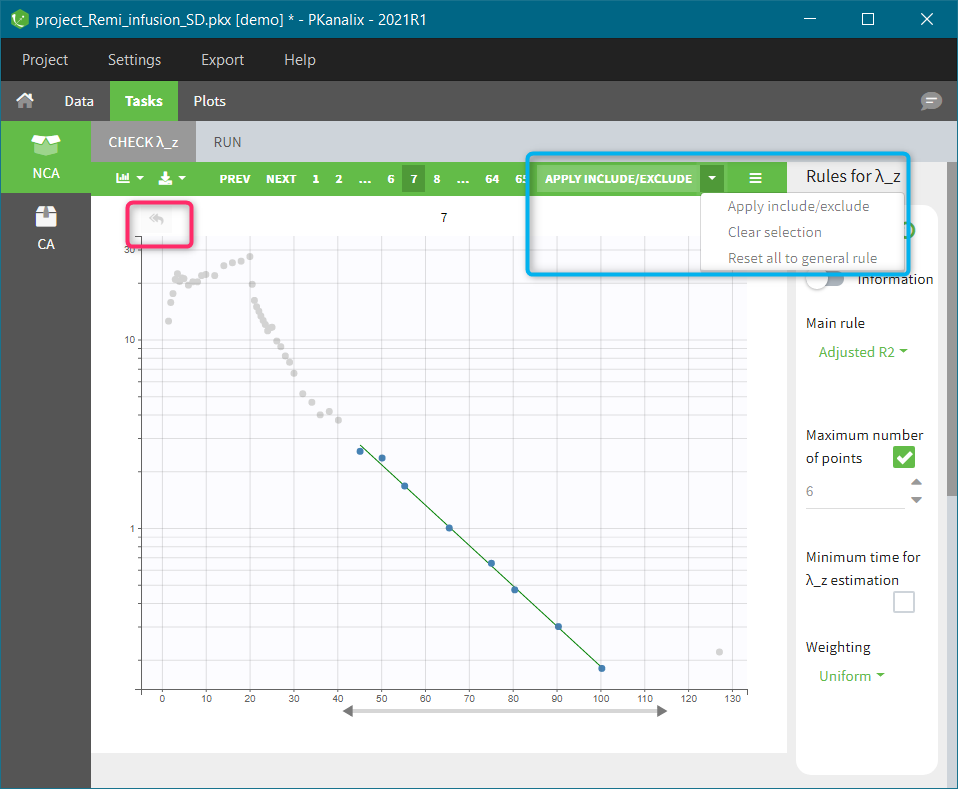
Include/exclude single points
It is possible to manually modify each point to include it in the calculation of \(\lambda_z\) or to remove it from the calculation:
- If you click on an unused point (light grey), it will change its color into light blue and will be selected for inclusion (figure on the left below).
- If you click on a used point (blue), it will change its color into dark grey and will be selected for exclusion (figure on the right below).
Clicking on the “Apply include/exclude” button applies these changes. The “return arrow” in the top – left corner of each individual plot resets the individual selection to the general rule one by one, while the “Reset to general rule” button in the “Apply include/exclude” drop-down menu resets all of them at once.
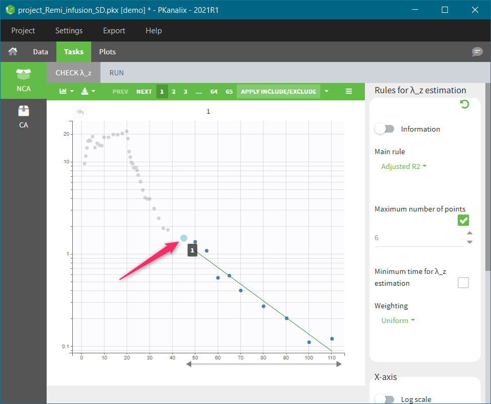 |
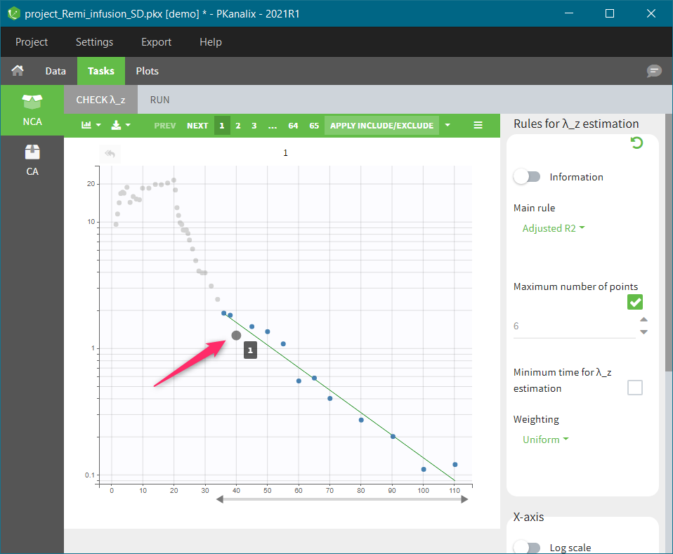 |
|---|
Remarks
- If the general rule is modified, only the individuals for which the general rule applies will be updated. Individual for which the points have been manually modified will not be updated.
- If the \(\lambda_z\) can not be computed, the background of the plot will be in red as in the following figure.
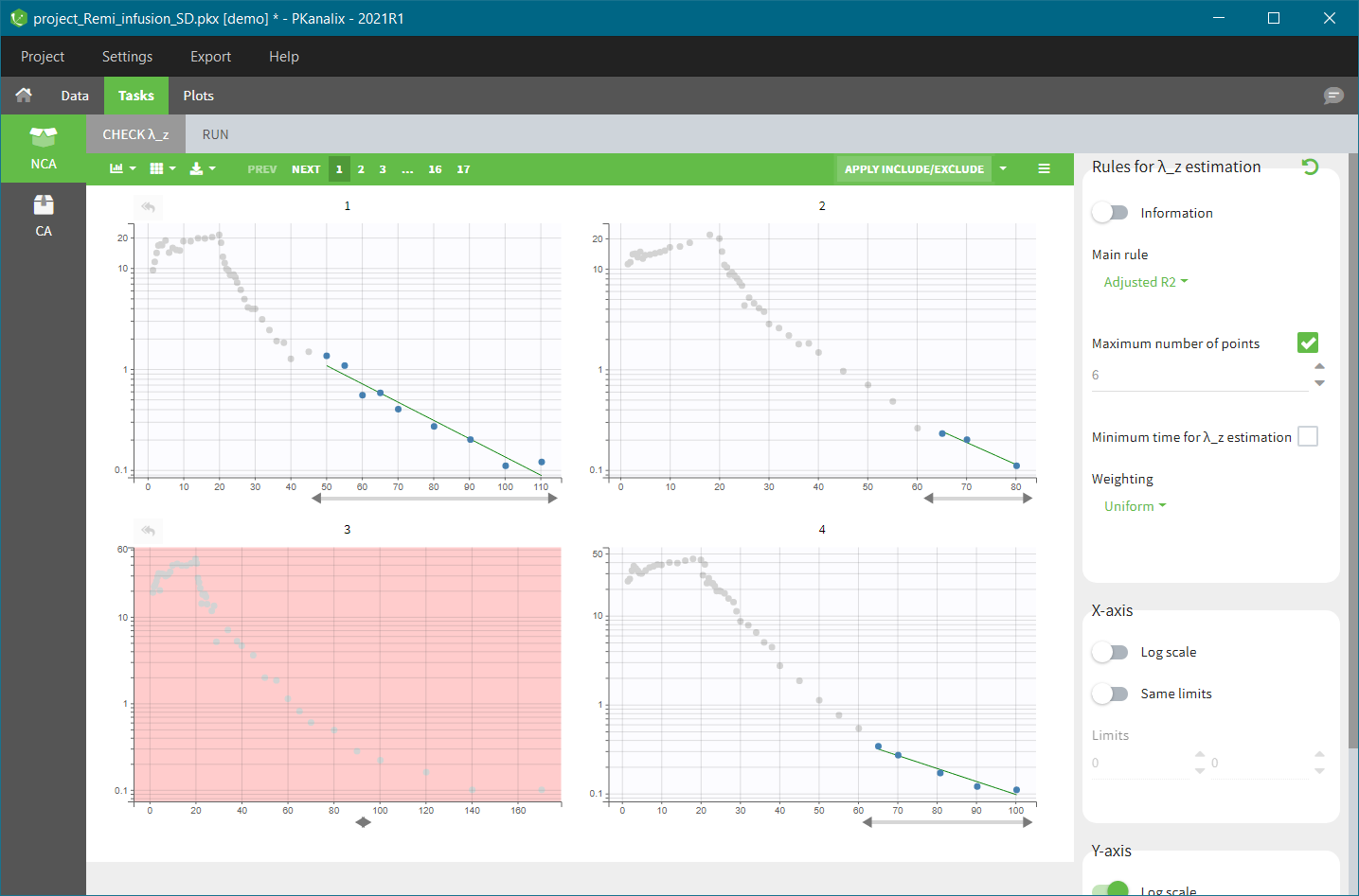
3.2.Data processing and calculation rules
This page presents the rules applied to pre-process the data set and the calculation rules applied for the NCA analysis.
Data processing
Ignored data
All observation points occurring before the last dose recorded for each individual are excluded. Observation points occurring at the same time as the last dose are kept, irrespective of their position in the data set file.
Note that for plasma data, negative or zero concentrations are not excluded.
Forbidden situations
For plasma data, mandatory columns are ID, TIME, OBSERVATION, and AMOUNT. For urine data, mandatory columns are ID, TIME, OBSERVATION, AMOUNT and one REGRESSOR (to define the volume).
Two observations at the same time point will generate an error.
For urine data, negative or null volumes and negative observations generate an error.
Additional points
For plasma data, if an individual has no observation at dose time, a value is added:
- Extravascular and Infusion data: For single dose data, a concentration of zero. For steady-state, the minimum value observed during the dosing interval.
- IV Bolus data: the concentration at dose time (C0) is extrapolated using a log-linear regression (i.e log(concentration) versus time) with uniform weight of first two data points. In the following cases, C0 is taken to be the first observed measurement instead (can be zero or negative):
- one of the two observations is zero
- the regression yields a slope >= 0
BLQ data
Measurements marked as BLQ data with a “1” in the CENSORING column will be replaced by zero, the LOQ value or the LOQ value divided by 2, or considered as missing (i.e excluded) depending on the setting chosen. They are then handled as any other measurement. The LOQ value is indicated in the OBSERVATION column of the data set.
Steady-state
Steady-state is indicated using the STEADY-STATE and INTERDOSE INTERVAL column-types. Equal dosing intervals are assumed. Observation points occurring after the dose time + interdose interval are excluded for Cmin and Cmax, but not for lambda_z. Dedicated parameters are computed such as the AUC in the interdose interval, and some specific formula should be considered for the clearance and the volume for example. More details can be found here.
Urine
Urine data is assumed to be single-dose, irrespective of the presence of a STEADY-STATE column. For the NCA analysis, the data is not used directly. Instead the intervals midpoints and the excretion rate for each interval (amount eliminated per unit of time) are calculated and used:
\( \textrm{midpoint} = \frac{\textrm{start time } + \textrm{ end time}}{2} \)
\( \textrm{excretion rate} = \frac{\textrm{concentration } \times \textrm{ volume}}{\textrm{end time } – \textrm{ start time}} \)
Calculation rules
Lambda_z
PKanalix tries to estimate the slope of the terminal elimination phase, called \( \lambda_z \), as well as the intercept called Lambda_z_intercept. \( \lambda_z \) is calculated via a linear regression between Y=log(concentrations) and the X=time. Several weightings are available for the regression: uniform, \( 1/Y\) and \(1/Y^2\).
Zero and negative concentrations are excluded from the regression (but not from the NCA parameter calculations). The number of points included in the linear regression can be chosen via the “Main rule” setting. In addition, the user can define specific points to include or exclude for each individual (see Check lambda_z page for details). When one of the automatic “main rules” is used, points prior to Cmax, and the point at Cmax for non-bolus models are never included. Those points can however be included manually by the user. If \( \lambda_z \) can be estimated, NCA parameters will be extrapolated to infinity.
R2 rule: the regression is done with the three last points, then four last points, then five last points, etc. If the R2 for n points is larger than or equal to the R2 for (n-1) points – 0.0001, then the R2 value for n points is used. Additional constrains of the measurements included in the \( \lambda_z \) calculation can be set using the “maximum number of points” and “minimum time” settings. If strictly less than 3 points are available for the regression or if the calculated slope is positive, the \( \lambda_z \) calculation fails.
Adjusted R2 rule: the regression is done with the three last points, then four last points, then five last points, etc. For each regression the adjusted R2 is calculated as:
\( \textrm{Adjusted R2} = 1 – \frac{(1-R^2)\times (n-1)}{(n-2)} \)
with (n) the number of data points included and (R^2) the square of the correlation coefficient.
If the adjusted R2 for n points is larger than or equal to the adjusted R2 for (n-1) points – 0.0001, then the adjusted R2 value for n points is used. Additional constrains of the measurements included in the \( \lambda_z \) calculation can be set using the “maximum number of points” and “minimum time” settings. If strictly less than 3 points are available for the regression or if the calculated slope is positive, the \( \lambda_z \) calculation fails.
Interval: strictly positive concentrations within the given time interval are used to calculate \( \lambda_z \). Points on the interval bounds are included. Semi-open intervals can be defined using +/- infinity.
Points: the n last points are used to calculate \( \lambda_z \). Negative and zero concentrations are excluded after the selection of the n last points. As a consequence, some individuals may have less than n points used.
AUC calculation
The following linear and logarithmic rule apply to calculate the AUC and AUMC over an interval [t1, t2] where the measured concentrations are C1 and C2. The total AUC is the sum of the AUC calculated on each interval. If the logarithmic AUC rule fails in an interval because C1 or C2 are null or negative, then the linear interpolation rule will apply for that interval.
Linear formula:
\( AUC |_{t_1}^{t_2} = (t_2-t_1) \times \frac{C_1+C_2}{2} \)
\( AUMC |_{t_1}^{t_2} = (t_2-t_1) \times \frac{t_1 \times C_1+ t_2 \times C_2}{2} \)
Logarithmic formula:
\( AUC |_{t_1}^{t_2} = (t_2-t_1) \times \frac{C_2 – C_1}{\ln(\frac{C_2}{C_1})} \)
\( AUMC |_{t_1}^{t_2} = (t_2-t_1) \times \frac{t_2 \times C_2 – t_1 \times C_1}{\ln(\frac{C_2}{C_1})} – (t_2-t_1)^2 \times \frac{C_2 – C_1}{\ln(\frac{C_2}{C_1})^2} \)
Interpolation formula for partial AUC
When a partial AUC is requested at time points not included is the original data set, it is necessary to add an additional measurement point. Those additional time points can be before or after the last observed data point.
Note that the partial AUC is not computed if a bound of the interval falls before the dosing time.
Additional point before last observed data point
Depending on the choice of the “Integral method” setting, this can be done using a linear or log formula to find the added concentration C* at requested time t*, given that the previous and following measurements are C1 at t1 and C2 at t2.
Linear interpolation formula:
\( C^* = C_1 + \left| \frac{t^*-t_1}{t_2-t_1} \right| \times (C_2-C_1) \)
Logarithmic interpolation formula:
\( C^* = \exp \left( \ln(C_1) + \left| \frac{t^*-t_1}{t_2-t_1} \right| \times (\ln(C_2)-\ln(C_1)) \right) \)
If the logarithmic interpolation rule fails in an interval because C1 or C2 are null or negative, then the linear interpolation rule will apply for that interval.
Additional point after last observed data point
If \( \lambda_z \) is not estimable, the partial area will not be calculated. Otherwise, \( \lambda_z \) is used to calculate the additional concentration C*:
\( C^* = \exp(\textrm{Lambda_z_intercept} – \lambda_z \times t) \)
Calculating steady-state parameters after each dose
Since version 2024R1, steady state parameters can be calculated for each profile without the dataset requiring the steady state information, meaning that the interdose-interval and SS columns are no longer necessarily. To enforce the calculation of steayd-state parameter (e.g AUC_TAU), the user must tick the NCA setting “Interdose interval for single dose profiles” and define a value for the inter-dose interval tau:
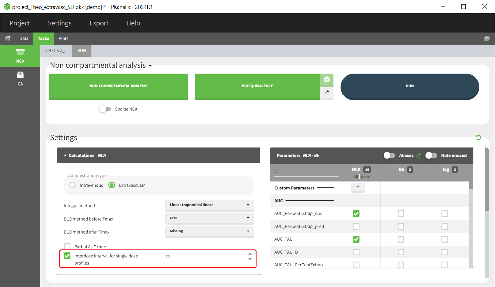
Single dose parameters are always calculated, irrespective of the presense or abscence of an inter-dose interval column in the dataset or whether the checkbox “Interdose interval for single dose profiles” is ticket or not.
Steady-state parameters are calculated for all individuals if the checkbox “Interdose interval for single dose profiles” is ticked (and a value for tau is defined). They are also calculated for individuals having a positive interdose interval is defined in the dataset or if the profile (subject or occasion) contains several doses. Deepnding on the dataset, you may have some profiles with steady-state parameters and some without (appearing as NaN in the results).
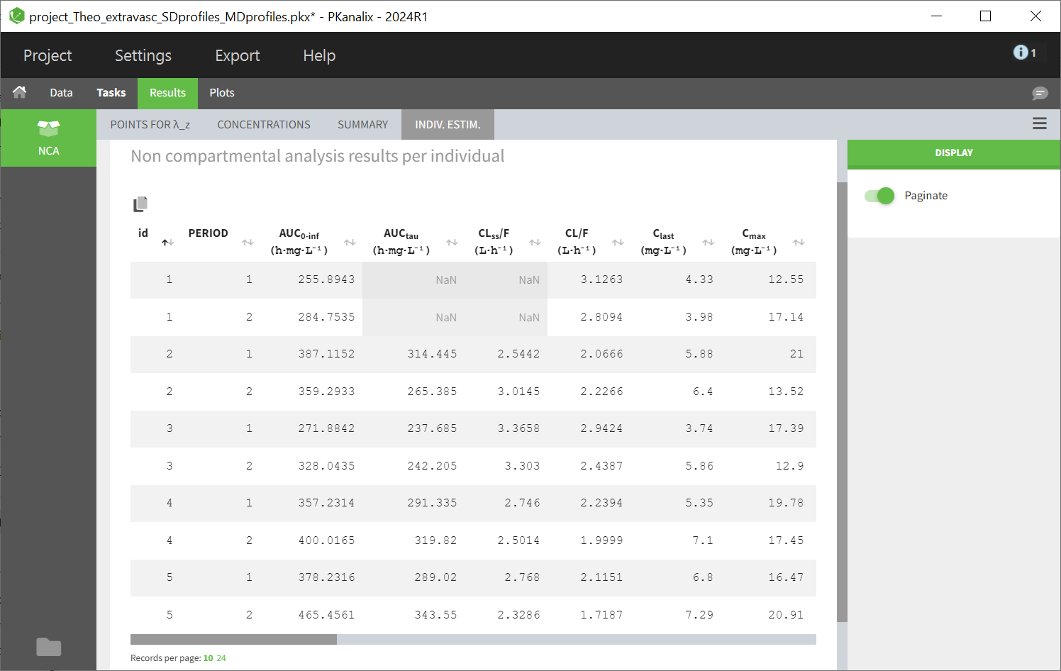
Some parameters have identical names but are computed using different formulas, contingent upon whether it pertains to a single dose profile or a multiple dose profile:
| Name | Formula/Description – SD | Formula/Description – SS |
|---|---|---|
| C0 | Concentration at dosing time. If profile doesn’t contain obs at dosing time: Extravascular or Infusion: C0 = 0. For IV bolus: log-linear regression of first two data points to back-extrapolate C0. | Minimum observed during the dose interval. |
| Cmax | Maximum observed concentration, occurring at Tmax. If not unique, then the first maximum is used. | Maximum observed concentration between dose time and dose time + TAU. |
| Cmax_D | Cmax/Dose | Cmax (based on SS)/Dose |
| Tmax | Time of maximum observed concentration; entire curve is considered. | Tmax corresponds to points collected during a dosing interval. |
| MRTINF_obs | Intravascular: MRTINF_obs = AUMCINF_obs/AUCINF_obs – TI/2; TI
infusion duration Extravascular: MRTINF_obs = AUMCINF_obs/AUCINF_obs → AUMCINF_obs & AUCINF_obs based on Clast_obs. |
Mean Residence Time extrapolated to infinity using predicted Clast, calculated using AUC_TAU. |
| MRTINF_pred | Same formulas as above but based on AUMCINF_pred & AUCINF_pred based on Clast_pred. | |
| Vss_obs | Vss_obs=MRTINF_obs * Cl_obs with MRTINF_obs for SD profiles | Vss_obs=MRTINF_obs * Cl_obs with MRTINF_obs for SS profiles |
| Vss_pred | Vss_pred=MRTINF_pred * Cl_pred with MRTINF_pred for SD profiles | Vss_pred=MRTINF_pred * Cl_pred with MRTINF_pred for SS profiles |
These parameters are distinguished by the postfix “_SS” in the list of parameters and in the results table. This extension is also echoed in the aliases by the postfix “, SS”.
Typically, parameters that share the same name are calculated differently based on whether the “Interdose interval for single dose profiles” checkbox is selected. However, there’s one exception: parameter C0. In cases where both single dose and multiple dose profiles occur together, the order of profiles influences C0‘s calculation. If the first profile is a single dose, followed by either more single dose profiles or multiple dose profiles, and the checkbox is enabled, C0 for the first occasion follows the single dose formula, while subsequent C0‘s follow the steady-state formula.
Ratios for NCA parameters
Starting from PKanalix version 2024R1 and above, ratios for each individual of NCA metrics along occasions can now be calculated. In the dedicated section “Ratios NCA” in the NCA tasks tab, ratios can be defined by clicking on the plus sign (red frame). This action prompts a window to appear, allowing you to specify the ratio in greater detail.
The ratio is calculated for each individual, using the different occasions (i.e profiles). When only one occasion corresponds to the modality selected for “ref” and “test”, the ratio is simply the ratio of the two values. If there are subjects who have multiple occasions corresponding to the modality selected for “ref” and “for “test”, the arithmetic mean of the values for this modality is calculated first, then the ratio is calculated.
If there are subjects without a parameter value for one of the test or comparison modalities, no ratio can be calculated for this parameter. Consequently, the subject obtains NaN as a result.
3.3.NCA settings
The following page describes all the settings for the parameters calculations.
- Calculations settings
- \(\lambda_z\) calculation settings
- Parameters to compute
- Acceptance criteria settings
- Ratios for NCA parameters
Calculations
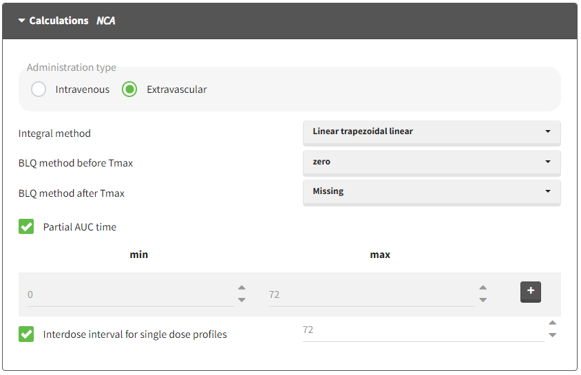
These settings corresponds to the settings impacting the calculation of the NCA parameters.
- Administration type: Intravenous or Extravascular. This defines the drug type of administration. IV bolus and IV infusions must be set as “intravenous”.
- Integral method: Method for AUC and AUMC calculation and interpolation. Trapezoidal refers to formula to calculate the AUC and Interpolation refers to the formula to add an additional point in case of partial AUC with a time point not originally present in the data set. See the Calculation rules for details on the formulas.
- Linear Trapezoidal Linear (Linear trapezoidal, linear interpolation): For AUC calculation linear formula. For interpolation linear formula.
- Linear Log Trapezoidal (Linear/log trapezoidal, linear/log interpolation): For AUC, linear before Cmax and log after Cmax. For interpolation, linear before Cmax and log after.
- Linear Up Log Down (LinUpLogDown trapezoidal, LinUpLogDown interpolation): For AUC, linear if concentration is going up or is stable, log if going down. For interpolation, linear if concentration is going up or is stable, log if going down.
- Linear Trapezoidal linear/log (Linear trapezoidal, linear/log interpolation): For AUC, linear formula. For interpolation, linear before Cmax, log after Cmax. If several Cmax, the first one is used.
For all methods, if an observation value is less than or equal to zero, the program defaults to the linear trapezoidal or interpolation rule for that point. Similarly, if adjacent observations values are equal to each other, the program defaults to the linear trapezoidal or interpolation rule.
- Partial AUC time: Define if the user would like to compute a partial AUC in a specific time interval. It is possible to define several partial AUC intervals, applicable to all individuals.
- BLQ before Tmax: In case of BLQ measurements, this corresponds to the method by which the BLQ data before Tmax should be replaced. Possible methods are “missing”, “LOQ”, “LOQ/2” or “0” (default value is 0).
- BLQ after Tmax: In case of BLQ measurements, this corresponds to the method by which the BLQ data after Tmax should be replaced. Possible methods are “missing”, “LOQ”, “LOQ/2” or “0” (default value is LOQ/2).
-
Interdose interval for single dose profiles: To compute steady-state parameters for single dose profiles, a value for \( \tau\) can be manually specified. The input value may be a double, under the condition that it is strictly positive. By default, the last time point of the initial single dose profile is set. This option is available with PKanalix version 2024R1 and above.
- Obs. ID to use: When several OBS ID are present in the data, an additional option to choose which Obs ID to use for perform the NCA analysis appears.
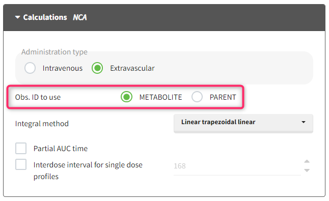
Settings impacting the \(\lambda_z\) calculation
This settings are impacting the calculation of \(\lambda_z\). See also the Check lambda_z page.
- Main rule for the \(\lambda_z\) estimation. It corresponds to the rule to define the measurements used for the \(\lambda_Z\) calculation. Possible rules are “R2”, “interval”, “points” or “adjustedR2” (called Best Fit in Winonlin) (default value is “adjustedR2”). See the calculation rules for more details.
- In case of “R2” or “adjustedR2” rule, the user has the possibility to define the maximum number of points and/or minimum time for the \(\lambda_z\) estimation. It allows to constrain the points tested for inclusion.
- In case of “Interval” rule, the user has the possibility to define the time interval to consider.
- In case of “Points” rule, the user has the possibility to define the number of points to consider.
- Weighting method used for the regression that estimates \(\lambda_z\). Possible methods are “Y”, “Y2” or “uniform” (default value is “uniform”).
Selecting NCA parameters to compute
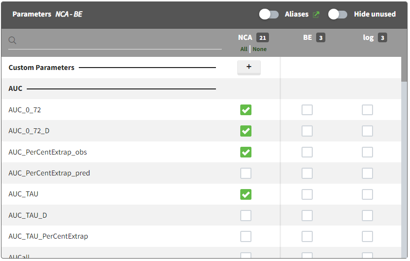
The NCA parameters to compute can be ticked in the “NCA” column. The list of NCA parameters is ordered by types of parameters. Custom NCA parameters can be defined using the “+” button.
It is recommended to always compute Rsq_adjusted, No_points_lambda_z, Lambda_z and Lambda_z_intercept as these parameters are necessary to display the terminal slope and information box in the NCA fit plot.
The list of parameters computed by default when starting a new PKanalix project can be defined in the Settings > Preferences.
Acceptance criteria
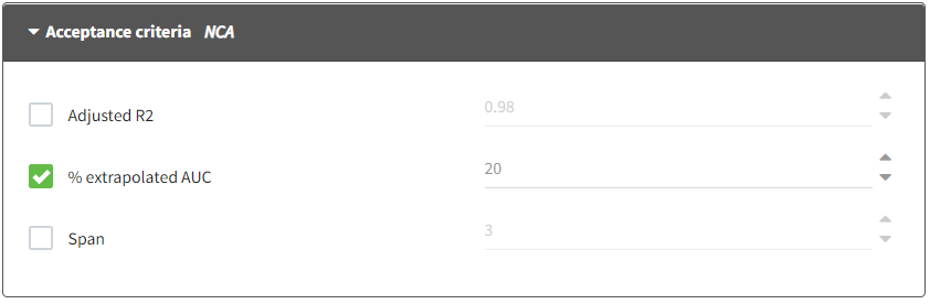
These settings corresponds to the settings impacting the acceptance criteria. When acceptance criteria are defined, flags indicating if the condition is met or not are added to the output result table. Statistics in the summary table can be calculated using only individuals who satisfy one or several acceptance criteria. The filtering option is available directly in the Summary sub-tab of the NCA results.
- Adjusted R2: It corresponds to the threshold of the adjusted R2 for the estimation of \(\lambda_z\). If activated, it will fill the value of Flag_Rsq_adjusted: if Rsq_adjusted > threshold, then Flag_Rsq_adjusted=1. The default value is .98.
- % extrapolated AUC: It corresponds to the threshold of the percentage of the total predicted AUC (or AURC for urine models) due to the extrapolation to infinity after the last measurement. If activated, it will fill the value of Flag_AUC_%Extrap_pred: if AUC_%Extrap_pred < threshold, then Flag_AUC_%Extrap_pred=1. The default value is 20%.
- Span: It corresponds to the threshold of the span. The span corresponds to the ratio of the sampling interval length for the \(\lambda_z\) calculation and the half-life. If activated, it will fill the value of Flag_Span: if Span > threshold, then Flag_Span=1. The default value is 3.
Ratios for NCA parameters
Starting from PKanalix version 2024R1 and above, ratios for each individual of NCA metrics along occasions can now be calculated. In the dedicated section “Ratios NCA” in the NCA tasks tab, ratios can be defined by clicking on the plus sign (red frame). This action prompts a window to appear, allowing you to specify the ratio in greater detail.
The Ratio definition box appears only if occasions are defined in the dataset.
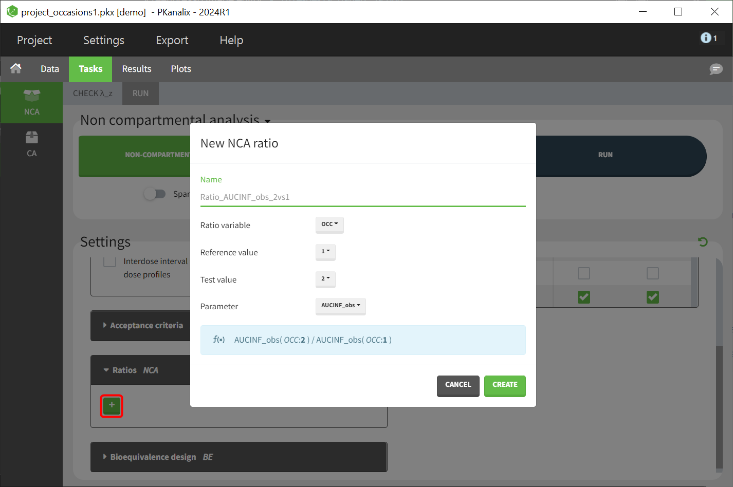
The definition is organised in several steps:
- Name: name for the new ratio parameter
- Ratio variable: Selection of the stratification variable. Variables tagged in the dataset either as occasion or as categorical variable are available for selection.
- Reference value: Selection of the reference modality (specific modality in Occasion or covariate vriable) to be used as denominator.
- Test value: Selection of test modality (specific modality in Occasion or covariate variable) to be used as numerator.
- Parameter: Selection of the NCA parameter
The formula for the specified ratio is displayed in the blue panel beneath the definition options.
Ratios can only be created using parameters that have been selected in the “NCA” column of the main parameter selection section.
For calculation details, see the Calculations rules page.
The computed parameter ratios are presented in two distinct results tables within the results tab. One table provides an individual listing, while the other offers a summary table with basic descriptive statistical metrics.
3.4.NCA parameters
The following page describes all the parameters computed by the non compartmental analysis. Parameter names are fixed and cannot be changed.
- Parameters related to \(\lambda_z\)
- Parameters related to plasma/blood measurements
- Parameters related to plasma/blood measurements specific to steady state dosing regimen
- Parameters related to urine measurements
- Parameters related to sparse NCA
- Parameter renamings
- Custom (user-defined) NCA parameters
Parameters related to \(\lambda_z\)
| Name | PKPARMCD CDISC | PKPARM CDISC | UNITS | DESCRIPTION |
|---|---|---|---|---|
| Rsq | R2 | R Squared | no unit | Goodness of fit statistic for the terminal (log-linear) phase between the linear regression and the data |
| Rsq_adjusted | R2ADJ | R Squared Adjusted | no unit | Goodness of fit statistic for the terminal elimination phase, adjusted for the number of points used in the estimation of \(\lambda_z\) |
| Corr_XY | CORRXY | Correlation Between TimeX and Log ConcY | no unit | Correlation between time (X) and log concentration (Y) for the points used in the estimation of \(\lambda_z\) |
| No_points_lambda_z | LAMZNPT | Number of Points for Lambda z | no unit | Number of points considered in the \(\lambda_z\) regression |
| Lambda_z | LAMZ | Lambda z | 1/time | First order rate constant associated with the terminal (log-linear) portion of the curve. Estimated by linear regression of time vs. log concentration |
| Lambda_z_lower | LAMZLL | Lambda z Lower Limit | time | Lower limit on time for values to be included in the \(\lambda_z\) calculation |
| Lambda_z_upper | LAMZUL | Lambda z Upper Limit | time | Upperlimit on time for values to be included in the \(\lambda_z\) calculation |
| HL_Lambda_z | LAMZHL | Half-Life Lambda z | time | Terminal half-life = ln(2)/Lambda_z |
| Lambda_z_intercept | – | – | no unit | Intercept found during the regression for (\lambda_z\), i.e. value of the regression (in log-scale) at time 0, i.e. the regression writes log(Concentration) = -Lambda_z*t+Lambda_z_intercept |
| Span | – | – | no unit | Ratio between the sampling interval of the measurements used for the \(\lambda_z\) and the terminal half-life = (Lambda_z_upper – Lambda_z_lower)*Lambda_z/ln(2) |
Parameters related to plasma/blood measurements
| Name | PKPARMCD CDISC | PKPARM CDISC | UNITS | DESCRIPTION |
|---|---|---|---|---|
| Tlag | TLAG | Time Until First Nonzero Conc | time | Tlag is the time prior to the first measurable (non-zero) concentration. Tlag is 0 if the first observation after the last dose is not 0 or LOQ. The value is set to 0 for non extravascular input. |
| T0 | time | Time of the dose | ||
| Dose | amount | Amount of the dose | ||
| N_Samples | – | – | no unit | Number of samples in the individuals. |
| C0 | C0 | Initial Conc | amount/volume | If a PK profile does not contain an observation at dose time (C0), the following value is added Extravascular and Infusion data. For single dose data, a concentration of zero. For steady-state, the minimum observed during the dose interval. IV Bolus data. Log-linear regression of first two data points to back-extrapolate C0. |
| Tmax | TMAX | Time of CMAX | time | Time of maximum observed concentration. – For non-steady-state data, the entire curve is considered. – For steady-state data, Tmax corresponds to points collected during a dosing interval. If the maximum observed concentration is not unique, then the first maximum is used. |
| Cmax | CMAX | Max Conc | amount/volume | Maximum observed concentration, occurring at Tmax. If not unique, then the first maximum is used. |
| Cmax_D | CMAXD | Max Conc Norm by Dose | 1/volume | Maximum observed concentration divided by dose. Cmax_D = Cmax/Dose |
| Tlast | TLST | Time of Last Nonzero Conc | time | Last time point with measurable concentration |
| Clast | CLST | Last Nonzero Conc | amount/volume | Concentration of last time point with measurable concentration |
| AUClast | AUCLST | AUC to Last Nonzero Conc | time.amount/volume | Area under the curve from the time of dosing to the last measurable positive concentration. The calculation depends on the Integral method setting. |
| AUClast_D | AUCLSTD | AUC to Last Nonzero Conc Norm by Dose | time/volume | Area under the curve from the time of dosing to the last measurable concentration divided by the dose. AUClast_D = AUClast/Dose |
| AUMClast | AUMCLST | AUMC to Last Nonzero Conc | time2.amount/volume | Area under the moment curve (area under a plot of the product of concentration and time versus time) from the time of dosing to the last measurable concentration. |
| MRTlast | MRTIVLST | MRT Intravasc to Last Nonzero Conc | time | [if intravascular] Mean residence time from the time of dosing to the time of the last measurable concentration, for a substance administered by intravascular dosing. MRTlast_iv = AUMClast/AUClast – TI/2, where TI represents infusion duration. |
| MRTlast | MRTEVLST | MRT Extravasc to Last Nonzero Conc | time | [if extravascular] Mean residence time from the time of dosing to the time of the last measurable concentration for a substance administered by extravascular dosing. MRTlast_ev = AUMClast/AUClast – TI/2, where TI represents infusion duration. |
| AUCall | AUCALL | AUC All | time.amount/volume | Area under the curve from the time of dosing to the time of the last observation. If the last concentration is positive AUClast=AUCall. Otherwise, AUCall will not be equal to AUClast as it includes the additional area from the last measurable concentration down to zero or negative observations. |
| AUCINF_obs | AUCIFO | AUC Infinity Obs | time.amount/volume | AUC from Dosing_time extrapolated to infinity, based on the last observed concentration. AUCINF_obs = AUClast + Clast/Lambda_z |
| AUCINF_D_obs | AUCIFOD | AUC Infinity Obs Norm by Dose | time/volume | AUCINF_obs divided by dose AUCINF_D_obs = AUCINF_obs/Dose |
| AUC_PerCentExtrap_obs | AUCPEO | AUC %Extrapolation Obs | % | Percentage of AUCINF_obs due to extrapolation from Tlast to infinity. AUC_%Extrap_obs = 100*(1- AUClast / AUCINF_obs) |
| AUC_PerCentBack_Ext_obs | AUCPBEO | AUC %Back Extrapolation Obs | % | Applies only for intravascular bolus dosing. the percentage of AUCINF_obs that was due to back extrapolation to estimate C(0). |
| AUMCINF_obs | AUMCIFO | AUMC Infinity Obs | time2.amount/volume | Area under the first moment curve to infinity using observed Clast AUMCINF_obs = AUMClast + (Clast/Lambda_z)*(Tlast + 1.0/Lambda_z) |
| AUMC_PerCentExtrap_obs | AUMCPEO | AUMC % Extrapolation Obs | % | Extrapolated (% or total) area under the first moment curve to infinity using observed Clast AUMC_%Extrap_obs = 100*(1- AUMClast / AUMCINF_obs) |
| MRTINF_obs | MRTIVIFO | MRT Intravasc Infinity Obs | time | [if intravascular] Mean Residence Time extrapolated to infinity for a substance administered by intravascular dosing using observed Clast MRTINF_obs_iv = AUMCINF_obs/AUCINF_obs- TI/2, where TI represents infusion duration. |
| MRTINF_obs | MRTEVIFO | MRT Extravasc Infinity Obs | time | [if extravascular] Mean Residence Time extrapolated to infinity for a substance administered by extravascular dosing using observed Clast MRTINF_obs_ev = AUMCINF_obs/AUCINF_obs |
| Vz_F_obs | VZFO | Vz Obs by F | volume | [if extravascular] Volume of distribution associated with the terminal phase divided by F (bioavailability) Vz_F_obs = Dose/Lambda_z/AUCINF_obs |
| Cl_F_obs | CLFO | Total CL Obs by F | volume/time | [if extravascular] Clearance over F (based on observed Clast) Cl_F_obs = Dose/AUCINF_obs |
| Vz_obs | VZO | Vz Obs | volume | [if intravascular] Volume of distribution associated with the terminal phase Vz_obs= Dose/Lambda_z/AUCINF_obs |
| Cl_obs | CLO | Total CL Obs | volume/time | [if intravascular] Clearance (based on observed Clast) Cl_obs = Dose/AUCINF_obs |
| Vss_obs | VSSO | Vol Dist Steady State Obs | volume | [if intravascular] An estimate of the volume of distribution at steady state based last observed concentration. Vss_obs = MRTINF_obs*Cl_obs |
| Clast_pred | – | – | amount/volume | Clast_pred = exp(Lambda_z_intercept- Lambda_z* Tlast) The values alpha (corresponding to the y-intercept obtained when calculating \(\lambda_z\)) and lambda_z are those values found during the regression for \(\lambda_z\) |
| AUCINF_pred | AUCIFP | AUC Infinity Pred | time.amount/volume | Area under the curve from the dose time extrapolated to infinity, based on the last predicted concentration, i.e., concentration at the final observation time estimated using the linear regression performed to estimate \(\lambda_z\) . AUCINF_pred = AUClast + Clast_pred/Lambda_z |
| AUCINF_D_pred | AUCIFPD | AUC Infinity Pred Norm by Dose | time/volume | AUCINF_pred divided by dose = AUCINF_pred/Dose |
| AUC_PerCentExtrap_pred | AUCPEP | AUC %Extrapolation Pred | % | Percentage of AUCINF_pred due to extrapolation from Tlast to infinity AUC_%Extrap_pred = 100*(1- AUClast / AUCINF_pred) |
| AUC_PerCentBack_Ext_pred | AUCPBEP | AUC %Back Extrapolation Pred | % | Applies only for intravascular bolus dosing. The percentage of AUCINF_pred that was due to back extrapolation to estimate C(0). |
| AUMCINF_pred | AUMCIFP | AUMC Infinity Pred | time2.amount/volume | Area under the first moment curve to infinity using predicted Clast AUMCINF_pred = AUMClast + (Clast_pred/Lambda_z)*(Tlast+1/Lambda_z) |
| AUMC_PerCentExtrap_pred | AUMCPEP | AUMC % Extrapolation Pred | % | Extrapolated (% or total) area under the first moment curve to infinity using predicted Clast AUMC_%Extrap_pred = 100*(1- AUMClast / AUMCINF_pred) |
| MRTINF_pred | MRTIVIFP | MRT Intravasc Infinity Pred | time | [if intravascular] Mean Residence Time extrapolated to infinity for a substance administered by intravascular dosing using predicted Clast |
| MRTINF_pred | MRTEVIFP | MRT Extravasc Infinity Pred | time | [if extravascular] Mean Residence Time extrapolated to infinity for a substance administered by extravascular dosing using predicted Clast |
| Vz_F_pred | VZFP | Vz Pred by F | volume | [if extravascular] Volume of distribution associated with the terminal phase divided by F (bioavailability) = Dose/Lambda_z/AUCINF_pred |
| Cl_F_pred | CLFP | Total CL Pred by F | volume/time | [if extravascular] Clearance over F (using predicted Clast) Cl_F_pred = Dose/AUCINF_pred |
| Vz_pred | VZP | Vz Pred | volume | [if intravascular] Volume of distribution associated with the terminal phas Vz_pred = Dose/Lambda_z/AUCINF_pred |
| Cl_pred | CLP | Total CL Pred | volume/time | [if intravascular] Clearance (using predicted Clast) = Dose/AUCINF_pred |
| Vss_pred | VSSP | Vol Dist Steady State Pred | volume | [if intravascular] An estimate of the volume of distribution at steady state based on the last predicted concentration. Vss_pred = MRTINF_pred*Cl_pred |
| AUC_lower_upper | AUCINT | AUC from T1 to T2 | time.amount/volume | AUC from T1 to T2 (partial AUC) |
| AUC_lower_upper_D | AUCINTD | AUC from T1 to T2 Norm by Dose | time/volume | AUC from T1 to T2 (partial AUC) divided by Dose |
| CAVG_lower_upper | CAVGINT | Average Conc from T1 to T2 | amount/volume | Average concentration from T1 to T2 |
Parameters related to plasma/blood measurements specific to steady state dosing regimen
In the case of repeated doses, dedicated parameters are used to define the steady state parameters and some specific formula should be considered for the clearance and the volume for example. Notice that all the calculation dedicated to the area under the first moment curve (AUMC) are not relevant.
| Name | PKPARMCD CDISC | PKPARM CDISC | UNITS | DESCRIPTION |
|---|---|---|---|---|
| Tau | – | time | The (assumed equal) dosing interval for steady-state data. | |
| Ctau | CTAU | Conc Trough | amount/volume | Concentration at end of dosing interval. If the observed concentration does not exist, the value is interpolated. It it cannot be interpolated, it is extrapolated using lambda_z. If lambda_z has not been computed, it is extrapolated as the last observed value. |
| Ctrough | CTROUGH | Conc Trough | amount/volume | Concentration at end of dosing interval. If the observed concentration does not exist, the value is NaN. |
| AUC_TAU | AUCTAU | AUC Over Dosing Interval | time.amount/volume | The area under the curve (AUC) for the defined interval between doses (TAU). The calculation depends on the Integral method setting. |
| AUC_TAU_D | AUCTAUD | AUC Over Dosing Interval Norm by Dose | time/volume | The area under the curve (AUC) for the defined interval between doses (TAU) divided by the dose. AUC_TAU_D = AUC_TAU/Dose |
| AUC_TAU_PerCentExtrap | – | – | % |
Percentage of AUC due to extrapolation in steady state.
AUC_TAU_%Extrap = 100*(AUC [Tlast, tau] if Tlast<=tau)/AUC_TAU;
|
| AUMC_TAU | AUMCTAU | AUMC Over Dosing Interval | time2.amount/volume | The area under the first moment curve (AUMC) for the defined interval between doses (TAU). |
| Vz_F | VZFTAU | Vz for Dose Int by F | volume | [if extravascular] The volume of distribution associated with the terminal slope following extravascular administration divided by the fraction of dose absorbed, calculated using AUC_TAU. Vz_F = Dose/Lambda_z/AUC_TAU |
| Vz | VZTAU | Vz for Dose Int | volume | [if intravascular] The volume of distribution associated with the terminal slope following intravascular administration, calculated using AUC_TAU. Vz = Dose/Lambda_z/AUC_TAU |
| CLss_F | CLFTAU | Total CL by F for Dose Int | volume/time | [if extravascular] The total body clearance for extravascular administration divided by the fraction of dose absorbed, calculated using AUC_TAU . CLss_F = Dose/AUC_TAU |
| CLss | CLTAU | Total CL for Dose Int | volume/time | [if intravascular] The total body clearance for intravascular administration, calculated using AUC_TAU. CLss = Dose/AUC_TAU |
| Cavg | CAVG | Average Concentration | amount/volume | AUCTAU divided by Tau. Cavg = AUC_TAU /Tau |
| FluctuationPerCent | FLUCP | Fluctuation% | % | The difference between Cmin and Cmax standardized to Cavg, between dose time and Tau. Fluctuation% = 100.0* (Cmax -Cmin)/Cavg |
| FluctuationPerCent_Tau | – | – | % | The difference between Ctau and Cmax standardized to Cavg, between dose time and Tau. Fluctuation% _Tau = 100.0* (Cmax -Ctau)/Cavg |
| Accumulation_Index | AILAMZ | Accumulation Index using Lambda z | no unit | Theoretical accumulation ratio: Predicted accumulation ratio for area under the curve (AUC) calculated using the Lambda z estimated from single dose data. Accumulation_Index = 1.0/(1.0 -exp(-Lambda_z*Tau)) |
| Swing | – | – | no unit | The degree of fluctuation over one dosing interval at steady state Swing = (Cmax -Cmin)/Cmin |
| Swing_Tau | – | – | no unit | Swing_Tau = (Cmax -Ctau)/Ctau |
| Tmin | TMIN | Time of CMIN observation. | time | Time of minimum concentration sampled during a dosing interval. |
| Cmin | CMIN | Min Conc | amount/volume | Minimum observed concentration between dose time and dose time + Tau. |
| Cmax | CMAX | Max Conc | amount/volume | Maximum observed concentration between dose time and dose time + Tau. |
| MRTINF_obs | MRTIVIFO or MRTEVIFO | MRT Intravasc Infinity Obs or MRT Extravasc Infinity Obs | time | Mean Residence Time extrapolated to infinity using predicted Clast, calculated using AUC_TAU. |
Parameters related to urine measurements
| Name | PKPARMCD CDISC | PKPARM CDISC | UNITS | DESCRIPTION |
|---|---|---|---|---|
| T0 | time | Time of the last administered dose (assumed to be zero unless otherwise specified). |
||
| Dose | – | – | amount | Amount of the dose |
| N_Samples | – | – | no unit | Number of samples in the individuals. |
| Tlag | TLAG | Time Until First Nonzero Conc | time | Midpoint prior to the first measurable (non-zero) rate. |
| Tmax_Rate | ERTMAX | Midpoint of Interval of Maximum ER | time | Midpoint of collection interval associated with the maximum observed excretion rate. |
| Max_Rate | ERMAX | Max Excretion Rate | amount/time | Maximum observed excretion rate. |
| Mid_Pt_last | ERTLST | Midpoint of Interval of Last Nonzero ER | time | Midpoint of collection interval associated with Rate_last. |
| Rate_last | ERLST | Last Meas Excretion Rate | amount/time | Last measurable (positive) rate. |
| AURC_last | AURCLST | AURC to Last Nonzero Rate | amount | Area under the urinary excretion rate curve from time 0 to the last measurable rate. |
| AURC_last_D | AURCLSTD | AURC to Last Nonzero Rate Norm by Dose | no unit | The area under the urinary excretion rate curve (AURC) from time zero to the last measurable rate, divided by the dose. |
| Vol_UR | VOLPK | Sum of Urine Vol | volume | Sum of Urine Volumes |
| Amount_Recovered | amount | Cumulative amount eliminated. | ||
| Percent_Recovered | % | 100*Amount_Recovered/Dose | ||
| AURC_all | AURCALL | AURC All | amount | Area under the urinary excretion rate curve from time 0 to the last rate. This equals AURC_last if the last rate is measurable. |
| AURC_INF_obs | AURCIFO | AURC Infinity Obs | amount | Area under the urinary excretion rate curve extrapolated to infinity, based on the last observed excretion rate. |
| AURC_PerCentExtrap_obs | AURCPEO | AURC % Extrapolation Obs | % | Percent of AURC_INF_obs that is extrapolated |
| AURC_INF_pred | AURCIFP | AURC Infinity Pred | amount | Area under the urinary excretion rate curve extrapolated to infinity, based on the last predicted excretion rate. |
| AURC_PerCentExtrap_pred | AURCPEP | AURC % Extrapolation Pred | % | Percent of AURC_INF_pred that is extrapolated |
| AURC_lower_upper | AURCINT | AURC from T1 to T2 (partial AUC) | amount | The area under the urinary excretion rate curve (AURC) over the interval from T1 to T2. |
| AURC_lower_upper_D | AURCINTD | AURC from T1 to T2 Norm by Dose | no unit | The area under the urinary excretion rate curve (AURC) over the interval from T1 to T2 divided by Dose |
| Rate_last_pred | – | – | amount/time | The values alpha and Lambda_z are those values found during the regression for lambda_z |
Parameters related to sparse NCA
| Name | UNITS | DESCRIPTION |
|---|---|---|
| SE_Cmax | amount/volume | Sample standard error of the concentration values at Tmax (standard deviation of the y-values at time Tmax divided by the square root of the number of observations at Tmax) |
| SE_AUClast | time.amount/volume | SE_AUClast = \(\sqrt{Var(\hat{AUC})} = \sqrt{\sum_{i=0}^{m} \frac{w_i^2s_i^2}{n_i}+2 \sum_{i<j} \frac{w_i w_j n_{ij} s_{ij}}{n_i n_j}}\)with \( w_{i} = \begin{cases} \frac{t_1-t_0}{2}, & \text{if i=0}\\ \frac{t_{i+1}-t_{i-1}}{2}, & \text{if i=1, …, m}\\ \frac{t_m-t_{m-1}}{2}, & \text{if i=m} \end{cases} \) and \( s_{ij} = \sum_{k=1}^{n_{ij}} \frac{(C_{ik}-\bar{C_i})(C_{jk}-\bar{C_j})}{(n_{ij}-1)+(1-\frac{n_{ij}}{n_i})(1-\frac{n_{ij}}{n_j})}\) where:
|
| SE_AUCall | time.amount/volume | Same as SE_AUClast with m = last observation time |
| SE_Max_Rate | amount/time | Same as SE_Cmax with excretion rates |
| SE_AURC_last | amount | Same as SE_AUClast with excretion rates |
| SE_AURC_all | amount | Same as SE_AUCall with excretion rates |
SE_AUClast, SE_AUCall, SE_AURC_last, SE_AURC_all are available only if the integral method is “linear trapezoidal linear” or “linear trapezoidal linear/log” (because the formula is based on linear calculation of AUC).
Parameter renamings
Starting from the 2023 version of MonolixSuite, default parameter names used in results tables and plots in the graphical user interface and reports do not match the names present in the Name column of the tables above. The names that are used can be customized in the NCA parameters renamings section of Preferences. The section contains two columns:
- Parameter – this column contains parameter names from the tables above,
- Alias – this column contains parameter names used in the interface and the values in cells can be changed.
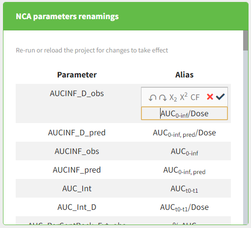
The Alias column is prefilled with default aliases. By clicking on an alias, PKanalix allows users to input characters. There are several options present, when in the input mode:
- Undo
 – reverse the last action,
 - Redo
 – redo an undone action,
 - Subscript
 – formats selected text and subsequently entered characters as subscript,
 - Superscript
 – formats selected text and subsequently entered characters as superscript,
 - CF
 – clears formatting of a selected text,
 - Cancel
 – cancels the changes and restores the alias,
 - Accept
 – accepts the changes (changes can be accepted by clicking anywhere in the interface as well).
3.5.Parameters summary
This pages provides the information on the statistics used for the summary of the individual parameters for both NCA tasks and CA tasks. All the statistics are made with respect to the NOBS individuals where the parameter has value. For example, in the NCA task, the parameter \(\lambda_z\) might not be possible to compute. Thus, the value associated to these subjects will be missing and not taken into account in the statistics.
- MIN: Minimum of the parameter over the NOBS individuals
- Q1: First quartile of the parameter over the NOBS individuals
- MEDIAN: Median of the parameter over the NOBS individuals
- Q3: Third quartile of the parameter over the NOBS individuals
- MAX: Maximum of the parameter over the NOBS individuals
- MEAN: Arithmetic mean of the parameter over the NOBS individuals
- SD: Standard deviation of the parameter over the NOBS individuals
- SE: Standard error of the parameter over the NOBS individuals
- CV: Coefficient of variation of the parameter over the NOBS individuals
- NTOT: Total number of individuals
- NOBS: Number of individuals with a valid value
- NMISS: Number of individuals with no valid value
- GEOMEAN: Geometric mean of the parameter over the NOBS individuals
- GEOSD: Geometric standard deviation of the parameter over the NOBS individuals
- GEOCV: Geometric coefficient of variation over the NOBS individuals
- HARMMEAN: Harmonic mean of the parameter over the NOBS individuals
3.6.Custom NCA parameters
- Definition via Preferences: user defined NCA parameters defined via Preferences can be used in any project with which they are compatible (if parameters that are used in the formula can be calculated in a project and if covariates used in the formula are present in the data set used in a project).
- Project-specific definition: user defined NCA parameters defined in a project will be used just in that particular project. However, when or after creating a project-specific NCA parameter, user can send the parameter to Preferences.
Definition of parameters
To define a parameter in Preferences, users can choose Settings > Preferences and define parameters in the section “NCA custom parameters”. To define project-specific parameters, users can click on the button “+” in the list of parameters in the Tasks tab.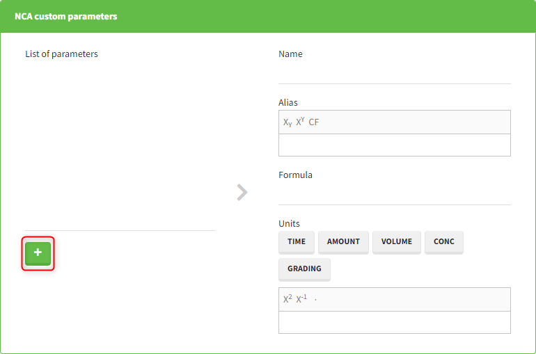
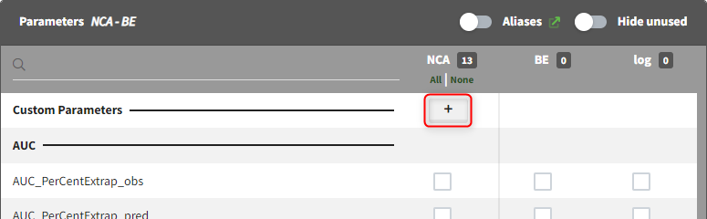
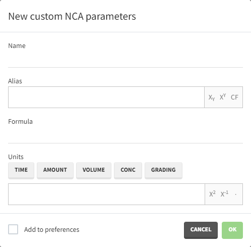
- Name: contains the name of the parameter used in the list of Parameters in the Tasks tab. This field can only start with a letter and cannot contain any special characters except “_”.
- Alias: parameter name used in results tables and plots in the graphical user interface and reports. Can contain special characters and can be stylized with subscripts and superscripts.
- Formula: mathematical expression used to define the parameter. The expression can contain NCA parameters calculated by PKanalix (list) and names of the covariates present in the data set. Operators +, –, *, /, and ^ can be used in the definition, as well as parentheses and functions abs, sqrt, exp, log, log10, logit, invlogit, sin, cos, tan, asin, acos, atan, sinh, cosh, tanh, floor, ceil, factorial, min, max, atan2, rem (definitions of those functions can be found here).
Partial AUC parameters can also be used in formulas, with slightly changed names – when start or end time contain a decimal point, it needs to be replaced by “d” (e.g., AUC_0_0.5 becomes AUC_0_0d5), and if they are in a scientific notation, a minus sign needs to be replaced by “m” (e.g., AUC_0_2e-10 becomes AUC_0_2em10).
When writing parameter names, an autocomplete panel will show up to help users write the name. If covariates are present in the project, instead of writing their names, users can click on the buttons available above the formula input field. - Units: contains the unit definition for the parameter. If a unit of a custom parameter depends on a project, generalized strings TIME, AMOUNT, VOLUME, CONC and GRADING can be used for time, amount, volume, concentration and dose normalization units defined in the project (these strings can be entered in a field via buttons above the field). Superscripts can be used with the syntax “^x” where x is a positive or a negative number (superscripts ^2 and ^-1 are also available via buttons). Different units can be concatenated using the character “.” (also available via a button). When defining a project-specific parameter, preview of the unit will be shown (the preview will replace the generalized strings with the units defined in the project). Note that “/” sign cannot be used. To define for instance “mg/L”, use “mg.L^-1”.
Custom parameter usage
The parameters defined via Preferences will appear in the dropdown of the Parameters section of the Tasks tab, if they are compatible with the current project (i.e if they use parameters that can be calculated for the current project and covariates present in the data set). They can be added to the project by clicking on them in the dropdown.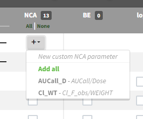
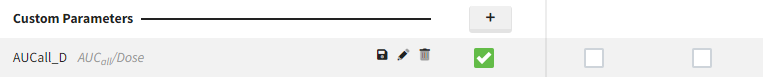
- Save in preferences () – available when a parameter is available in the project, but is not saved in the preferences (for example, the parameter was created in the project and the “Add to preferences” checkbox was not ticked, or the project was shared with a user that does not have the custom parameter in the preferences).
- Edit () – allows to edit the name, alias, formula and unit of a parameter. If a parameter is saved in the preferences, users will be asked if they want to update the parameter only in the current project, or also in the preferences.
- Delete () – removes the parameter from the project (but not from the preferences, if the parameter is saved in preferences).
3.7.Sparse NCA
Sparse data are data that have few observations per individual or per occasion, and that may not allow to estimate individual pharmacokinetic parameters reliably. Sparse data require specific handling in NCA analysis to get the most informative metrics from the data. PKanalix offers a dedicated mode to perform NCA analysis on sparse data, based on the calculation of mean profiles and standard errors of NCA parameters.
- Set up of sparse NCA
- Calculation of mean profiles
- NCA parameters specific to sparse data
- Sparse NCA results
Set up of sparse NCA
To specify a sparse dataset, you need to go to the NCA tab and select the “Sparse NCA” toggle below the NCA task. This will enable the calculation of mean profiles based on the individual data.
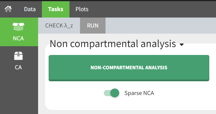
Sparse NCA is available for plasma and urine datasets.
Stratified sparse data
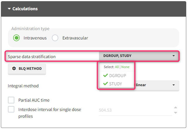
With the “Sparse data stratification” in NCA calculation settings, you can select one or more stratification covariates to group the data by different categories. For example, if you have a categorical covariate indicating the treatment group, you can select it to calculate a mean profile for each treatment group. The stratification covariates must be of type “categorical covariate” or “stratification categorical covariate” in the dataset tagging.
BLQ samples
If you have censored data, you can also click on the “BLQ method” button to select a censoring rule to handle the below limit of quantification (BLQ) samples.
The available rules are:
- Single rule: Replace all BLQ samples by [missing/zero/LOQ/(LOQ/2)]
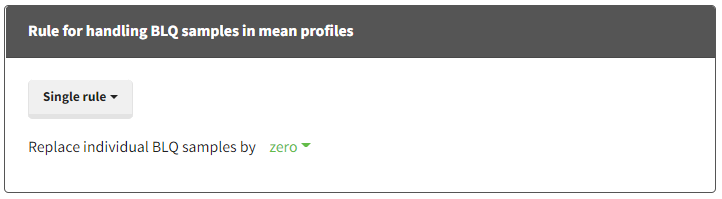
- Two rules based on absolute number of BLQ samples:
if Nblq >= [number]:- then:
- either replace BLQ samples by [missing/zero/LOQ/(LOQ/2)]
- or replace the mean sample by [missing/zero/LOQ/(LOQ/2)]
- else replace BLQ samples by [missing/zero/LOQ/(LOQ/2)]
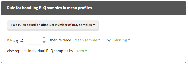
- then:
- Two rules based on fraction of total number of samples:
if Nblq >= [number] % of Ntot- then:
- either replace BLQ samples by [missing/zero/LOQ/(LOQ/2)]
- or replace the mean sample by [missing/zero/LOQ/(LOQ/2)]
- else replace BLQ samples by [missing/zero/LOQ/(LOQ/2)]

- then:
In addition, it is possible to check if the mean is below a LOQ value and add a special handling is it is the case:
- Check that mean samples stay above the LOQ:
If the mean sample is below [number] (LOQ usually), replace the mean sample by [missing/zero/LOQ/(LOQ/2)] before Tmax and [missing/zero/LOQ/(LOQ/2)] after Tmax.
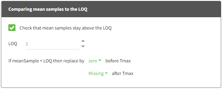
Read details on the calculations performed by these rules
- “Replace individual BLQ samples by [missing/zero/LOQ/(LOQ/2)]” = replace each individual censored sample by Missing (ie ignore the sample), LOQ (from the dataset for each sample) or LOQ/2.
- “If NBLQ > 33% of NTOT”: this condition is checked at each nominal time point and for each stratification group: NTOT is the total number of samples considered corresponding to that nominal time point and that stratification group, and NBLQ is the number of censored samples among them.
- “Replace mean sample by [missing/zero/LOQ/(LOQ/2)]” = replace the mean sample by Missing (ie ignore the mean sample in the mean profile), LOQ (largest LOQ found in the dataset among the censored samples involved in this mean sample), or LOQ/2.
- “Check that mean samples stay above the LOQ”: here the LOQ is the global LOQ value entered by the user in these settings.
- “If meanSample < LOQ then replace by LOQ”: here the LOQ in the condition and the replacement is the global LOQ value entered by the user in these settings.
Calculation of mean profiles
When “Sparse NCA” is selected, one or several mean profiles are calculated:
- One mean profile per stratification group is calculated (one group for each combination of modalities from the covariates selected in “Sparse stratification”).
- The mean profile is calculated by taking the mean concentration value across all subject-occasions for each unique time value for plasma data, or the mean rate value for each unique midpoint for urine data.
- If a column of type NOMINAL TIME is selected, the mean profiles are calculated based on nominal time, otherwise they are calculated based on TIME.
- If the individuals used to calculate a mean profile have different dosing regimen (different dosing time or dosing amount), only the dosing regimen from the first individual is kept for the mean profile.
- For urine data, if the individuals used to calculate a mean profile have different volumes for some interval, only the volumes from the first individual are kept for the mean profile.
- Subject-occasions are handled independently for the calculation of mean profiles.
The mean profiles do not appear in the Observed data plot, but they appear in Check lambda_z and NCA individual fits
NCA parameters specific to sparse data
All usual NCA parameters are available in the list of parameters to compute, and in addition the following NCA parameters are available:
- For plasma data: SE_Cmax, SE_AUClast, SE_AUCall
- For urine data: SE_Max_Rate, SE_AURC_last, SE_AURC_all
See the page on NCA parameters for more details.
These parameters are not selected by default. SE_AUClast, SE_AUCall, SE_AURC_last, SE_AURC_all are available only if the integral method is “linear trapezoidal linear” or “linear trapezoidal linear/log” (because the formula is based on linear calculation of AUC).
Sparse NCA results
The results of the NCA analysis on sparse data are displayed in the Results and Plots tabs. The table below summarizes the availability of the results in sparse NCAmode.
| Result | Based on |
| Tables of NCA parameters | mean profiles |
| Table of concentrations | individual data + mean profiles |
| NCA data plot | individual data + mean profiles |
| NCA individual fits | mean profiles |
| Other NCA plots | disabled |
The parameters calculated on the mean profiles appear in the table of individual NCA parameters and the NCA summary table.
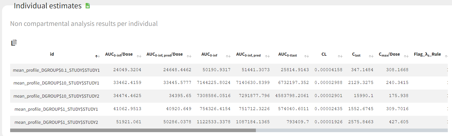
The table of concentrations displays both the individual concentration data, and the mean profiles on the “mean” rows. The table is stratified by the covariates selected for sparse data.
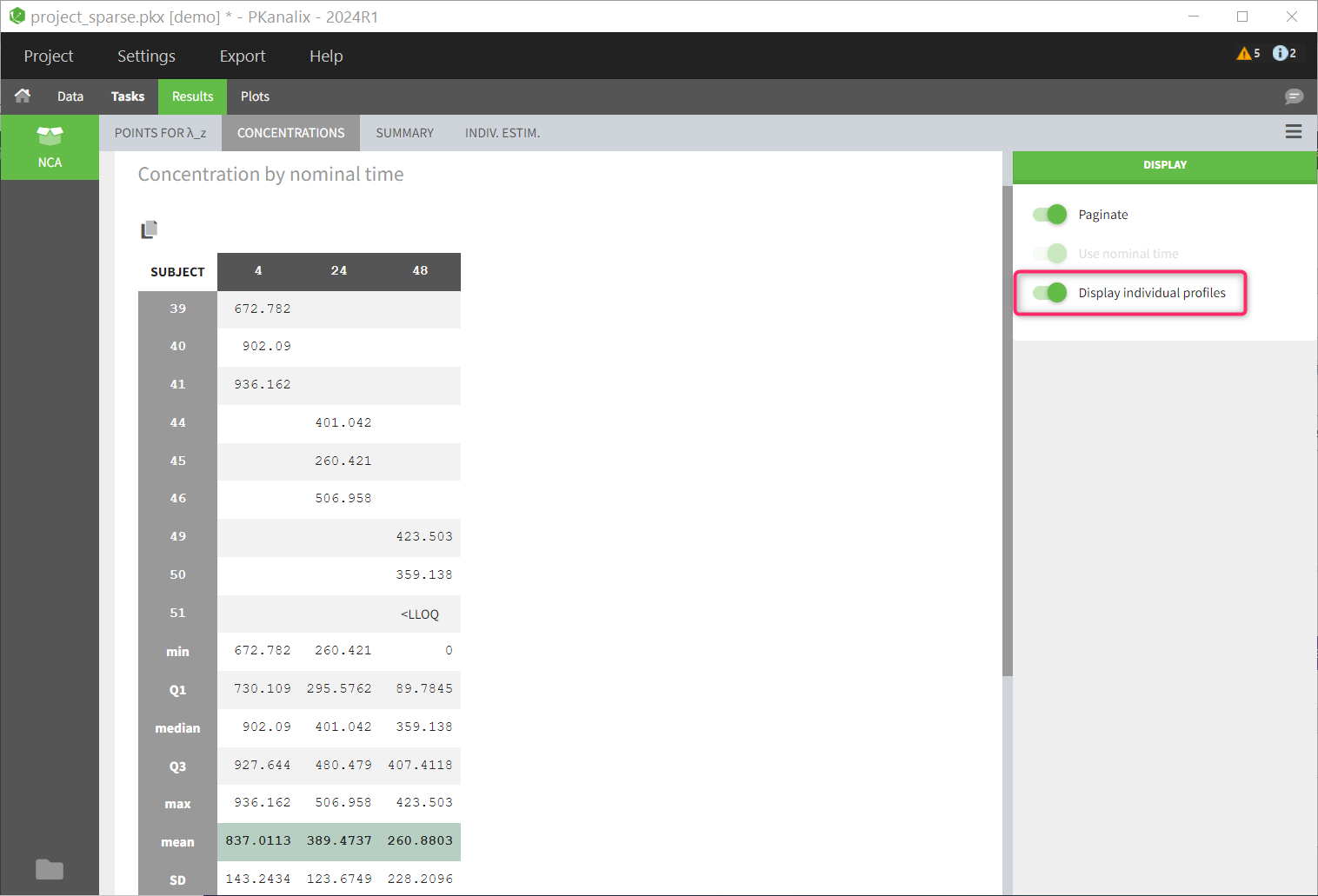
The NCA data plot is a new plot that shows the mean profiles and the individual data points on the same plot, with different colors for the different mean profiles.
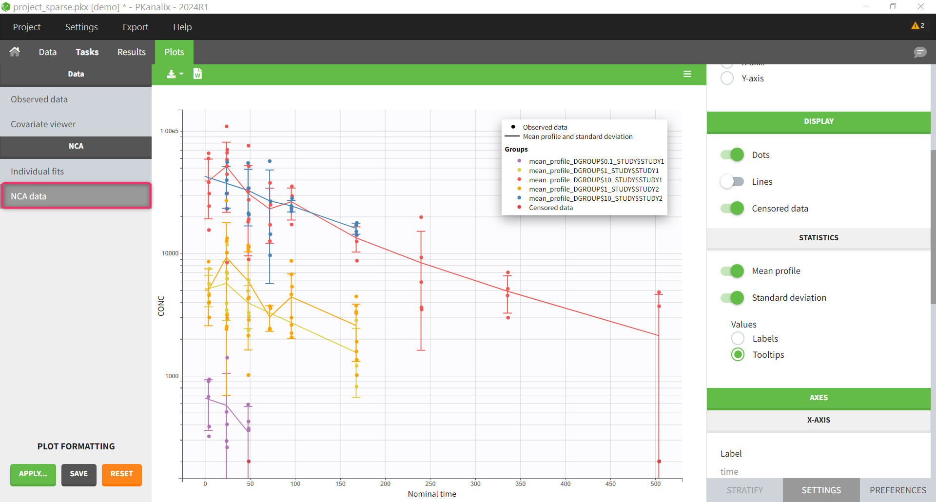
The NCA individual fits plot shows the mean profiles and the NCA parameters calculated on them. The other NCA plots are disabled because they are not relevant for sparse data analysis.
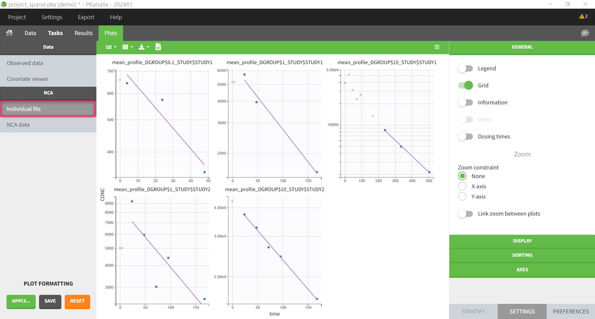
4.Compartmental Analysis
Overview of the workflow
One of the main features of PKanalix is the calculation of the parameters in the compartmental analysis framework. It find parameters of a compartmental model representing the PK dynamics for each individual using the Nelder-Mead algorithm.
NEW: PKanalix 2023 version performs individual model fit using any model with continuous outputs – loaded from the built-in library or a custom model.
Compartmental analysis workflow includes:
CA task
To access the compartmental analysis task in PKanalix use a dedicated section (left panel) in the “Tasks” tab, as in the following figure.
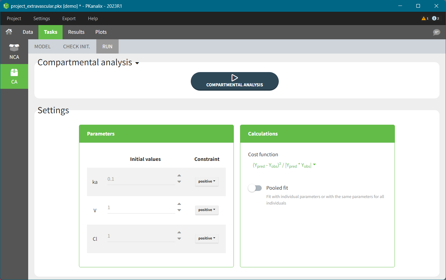
This task contains three sub-tabs:
- The first one called “MODEL” allows to select a model, e.g. from a PKanalix models library or your directory, edit it and match the observations from a dataset with model outputs. Complete guide to model definition is in the CA model page.
- The second one called “CHECK INIT.” shows model predictions obtained with the initial parameter values for each individual together with the data points. It helps to initialize model parameters by changing values manually or using the Auto-init function, as explained in the Initialization page.
- The third one called “Run” contains a button to run the calculations and the settings for the model and the calculations. The meaning of all the settings and their default values is defined the Settings page.
CA model
In this section you specify a model. You can edit the selected model directly in the interface. The right hand side section is to match observations from a dataset with model outputs, see here for a complete guide.
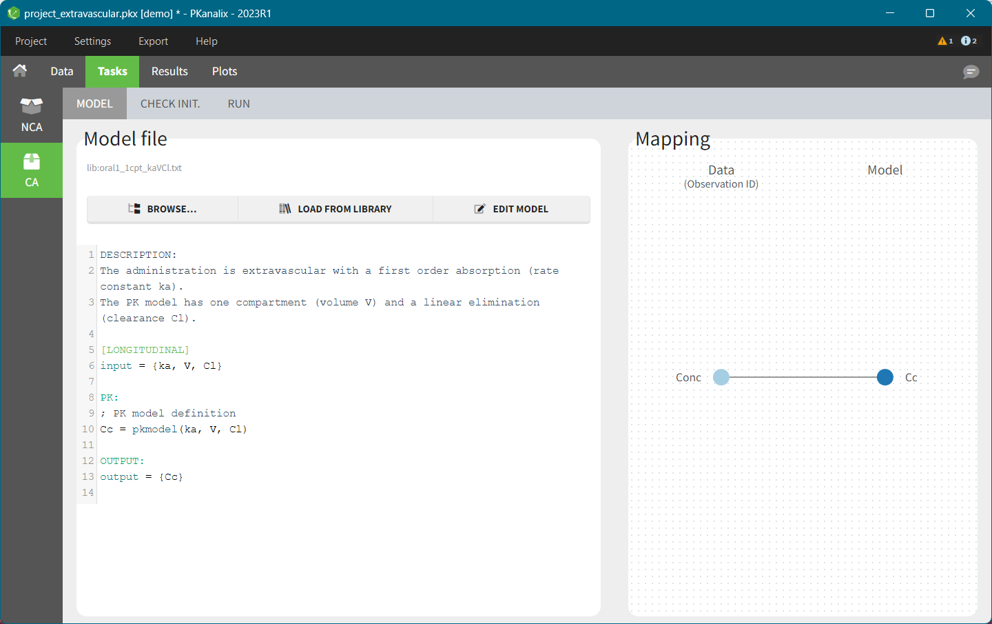
PKanalix accepts custom models – select BROWSE and load a .txt file with the model. There are also built-in libraries (PK, PK double absorption, TMDD, parent – metabolite, etc.), to facilitate the use of the software. Note that models can include multiple outputs. Models used in all MonolixSuite applications have to be in the mlxtran language. Note: For PKanalix versions before 2023, only the classical PK models, from the PK model library, are available.
CA check init.
The “Check init” tab helps to initialize model parameters. It shows the model predictions obtained with the initial model parameter values and the individual designs (doses and regressors). Each sub plot shows one individual with overlaid individual data points. This feature is very useful to find “good” initial values, as explained here.
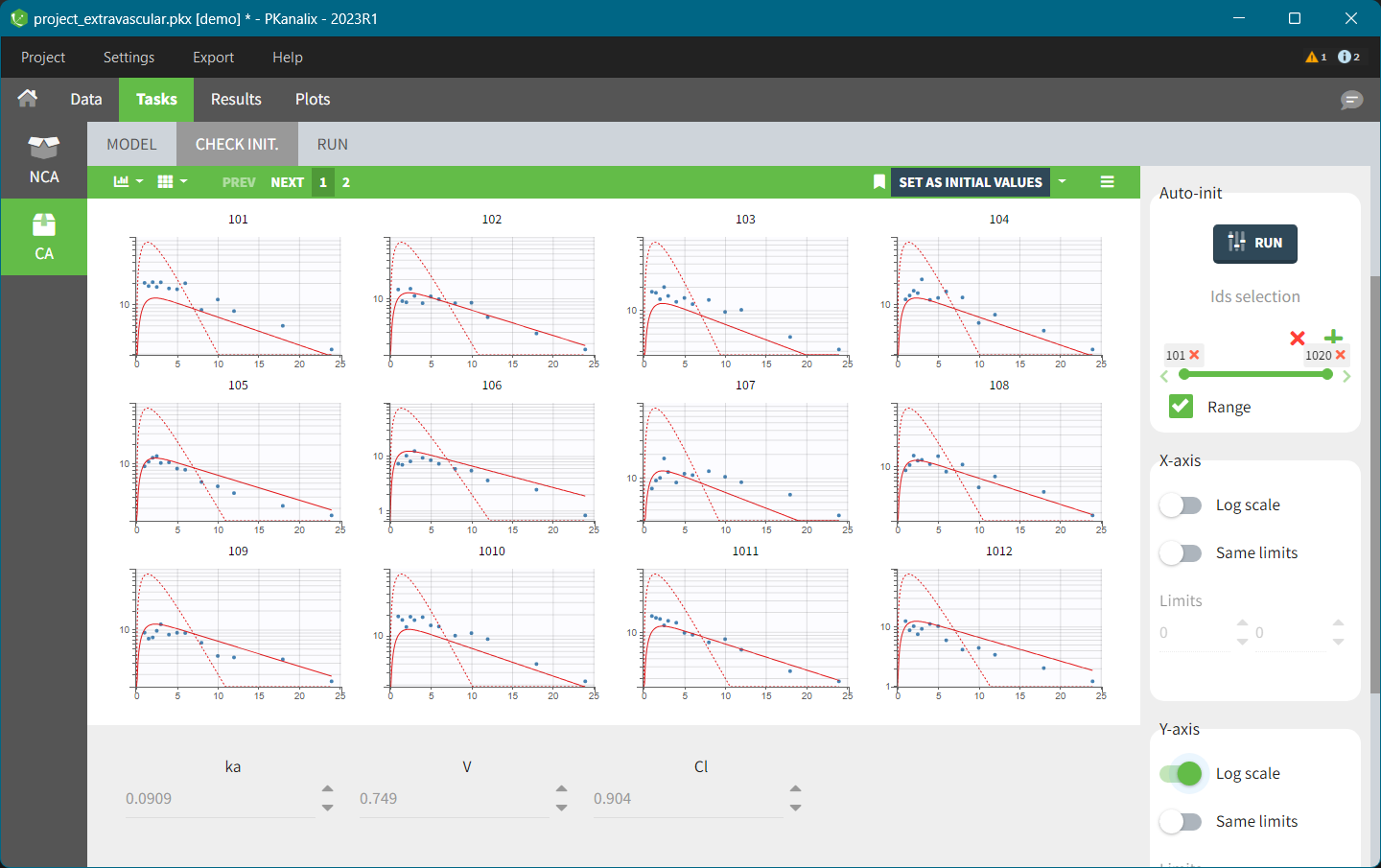
CA results
When you run the CA task, Pkanalix shows automatically the results in the “Results” tab, see the CA Results page for a complete guide. There are three tables:
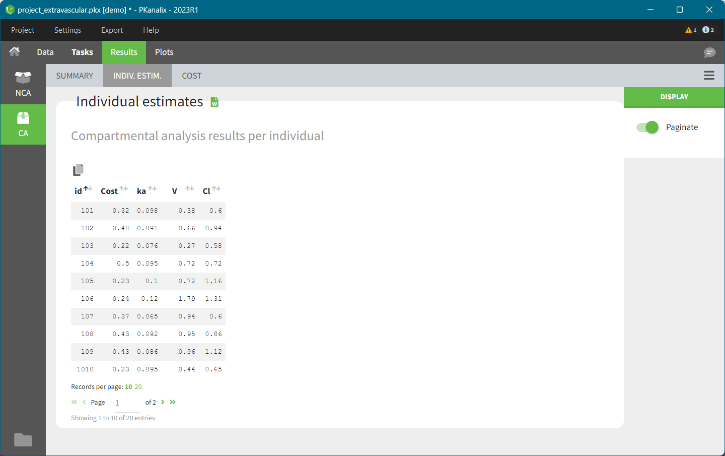
- INDIV. ESTIM contains compartmental analysis results for each individual.
- SUMMARY contains statistics on compartmental analysis results and summary calculation (described here). You can split or filter this table by covariates present in a dataset.
- COST contains cost function information.
All the computed parameters depend on the chosen model. To copy a table and paste in a word or an excel document click on the icon on the top left corner of a table.
CA plots
After running the CA task, several plots associated to the individual parameters are automatically generated and displayed In the “Plots” tab.
- Individual fits: displays model fit for each individual on a separate plot.
- Correlation between CA parameters: displays scatter plots for each pair of parameters and allows to identify correlations between parameters.
- Distribution of the CA parameters: displays the empirical distribution of the parameters and allows to analyse their distribution over the individuals.
- CA parameters w.r.t. covariates: displays the individual parameters as a function of the covariates and allows to identify correlation effects between the individual parameters and the covariates.
- Observations vs predictions displays observations from a dataset versus model predictions computed using individual parameters and is useful to detect misspecifications in the model.
CA outputs
After running the CA task, the following files are automatically generated in the project Result folder/IndividualParameters/ca :
- summary.txt contains the summary of the CA parameters calculation, in a format easily readable by a human (but not easy to parse for a computer).
- cost.txt contains the information about total cost and information criteria for a current model.
- caIndividualParametersSummary.txt contains the summary of the CA parameters in a computer friendly format useful for post-processing:
- The first column corresponds to the name of the parameters.
- The other columns correspond to the several elements describing the summary of the parameters (as explained here).
- caIndividualParameters.txt contains the CA parameters for each subject-occasion along with the covariates.
-
- The first line corresponds to the name of the parameters.
- The other lines correspond to the value of the parameters.
-
You can export the files caIndividualParametersSummary.txt and caIndividualParameters.txt in R for example using the following command
read.table("/path/to/file.txt", sep = ",", header = T)
Remark: the separator is the one defined in the user preferences. We set “,” in this example as it is the one by default.
CA export to Monolix/Simulx
Using the top menu “Export”, a PKanalix project (dataset information, model, estimated parameters) can be exported to Monolix or Simulx for further analysis, see Export to Monolix/Simulx page for a complete guide.
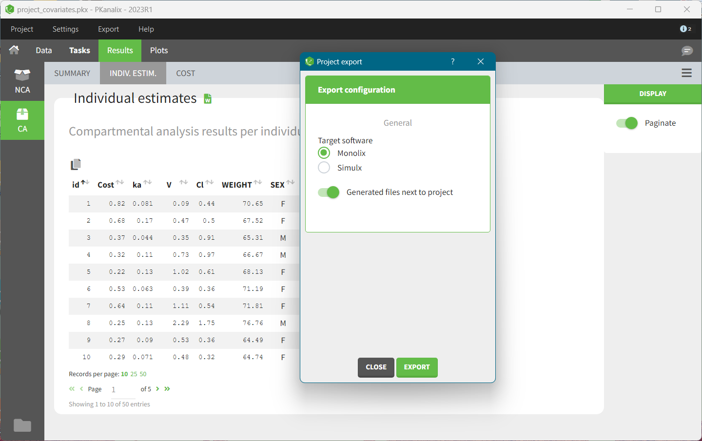
- Monolix for population modeling and further model development and diagnosis.
- Simulx to use a CA model and estimated individual parameters for simulations of new scenarios, eg. new dosing regimens.
Note: For PKanalix versions before 2023, only export to Monolix is available.
Next section: CA model
4.1.CA model
The first step to run the compartmental analysis task in PKanalix is selecting a model. Models in PKanalix are .txt files and are loaded in the Model sub tab of the Task tab. You can:
- Load a custom model from your directory by clicking the BROWSE button.
- Load a model from PKanalix library by clicking the LOAD FROM LIBRARY button.
- Write a new model from scratch in the mlxtran language by clicking the NEW MODEL button.
Note: In PKanalix versions before 2023, only models from the PK library are available.
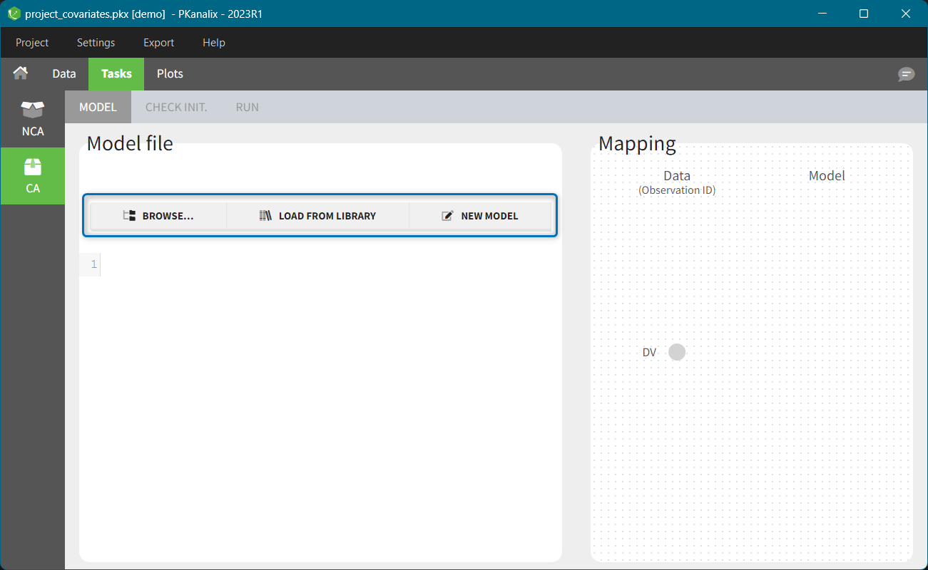
After loading a model, PKanalix switches automatically the MODEL sub-tab to the CHECK INIT. sub-tab for parameters initialization. To view the model file go back to the MODEL sub-tab. The left section shows the model file content. Clicking on the EDIT MODEL button allows to edit the model, save and apply it to the current project. For more details, see the custom model documentation page.The right hand side shows the mapping between the data set observations ids and the model outputs. For more details, see the mapping in Monolix documentation page. This feature is the same in PKanalix and Monolix.
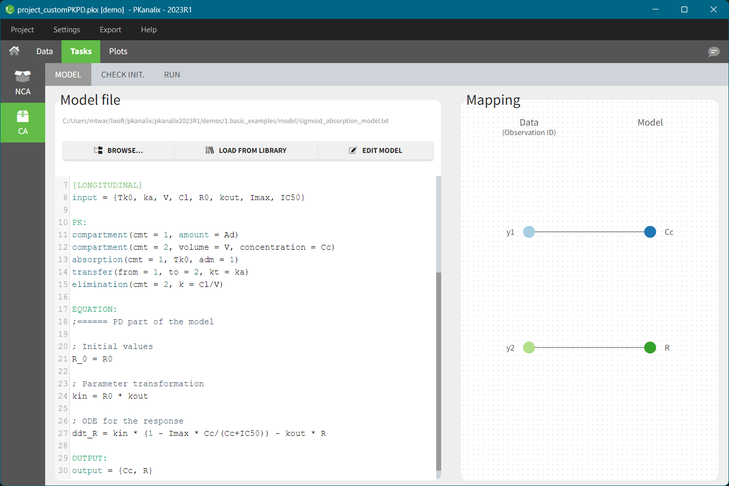
Saving model information in the PKanalix project file
In PKanalix, a model file is a .txt file and its name is displayed on top of the MODEL sub-tab. If a model is from the PKanalix library, then the file name contains a prefix “lib:”. For custom models there is the full path to the file.
Remark on using custom models. Be careful when you change a location of a model file. If it was used in any PKanalix project, then you will not be able to re-open this project. You will see an error “Missing model file at ‘original_path_to_modelFile/model_filename.txt’.”. To avoid such situation, use a project settings (In the top menu “Settings”) and switch on the toggle “Save the dataset and the model beside the project”.
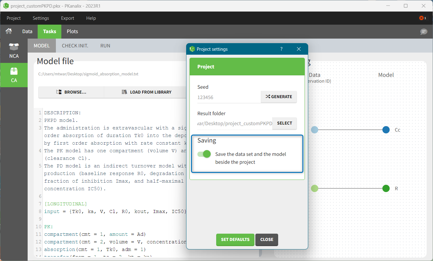
Next section: library of models
4.1.1.Libraries of models
PKanalix provides libraries of ready-to-use models for compartmental analysis. This simplifies the use of the software by decreasing the necessity of coding. You can pick models from the libraries, use them directly or edit. They are accessible in the Model sub-tab of the CA task by clicking the button “LOAD FROM LIBRARY“.
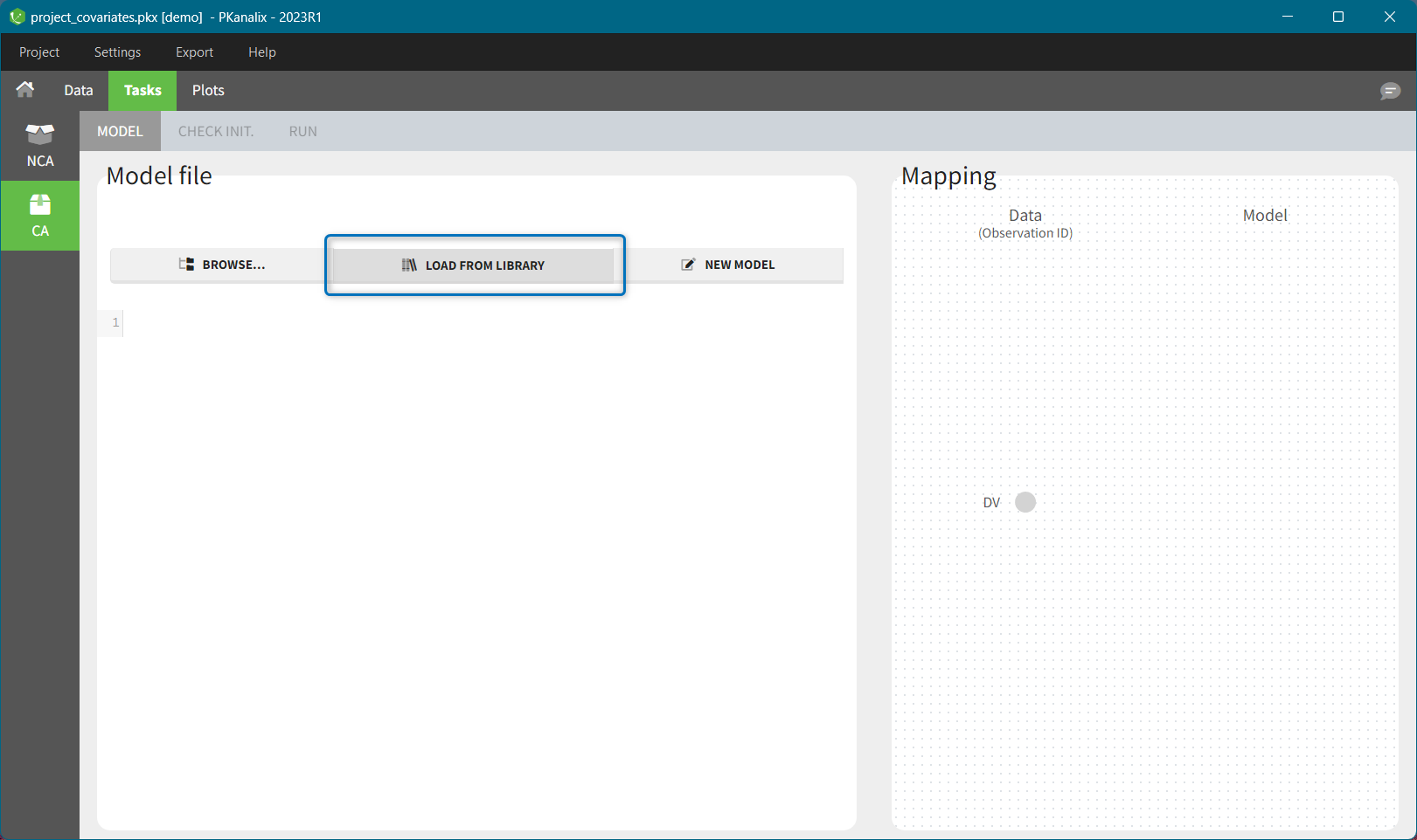
Libraries are organized into several categories:
- PK model library includes standard compartmental models. It is possible to select different administration routes (bolus, infusion, first-order absorption, zero-order absorption, with or without Tlag), different number of compartments (1, 2 or 3 compartments), and different types of eliminations (linear or Michaelis-Menten). The PK library models can be used with single or multiple doses data, and with two different types of administration in the same data set (oral and bolus for instance).
- PD model library includes direct response models such as Emax and Imax with various baseline models, and turnover response models. These models are PD models only and the drug concentration over time must be defined in the data set and passed as a regressor.
- PK/PD model library provides all standard combinations of pharmacokinetic and pharmacodynamic models.
- PK double absorption model library includes double absorption models. They take into account all the combinations of absorption types and delays for two absorptions. The absorptions can be specified as simultaneous or sequential, and with a pre-defined or independent order.
- Parent-Metabolite model library includes models describing parent drug and one metabolite, with or without the first pass effect, uni and bidirectional transformation and up to three compartments for parent and metabolite.
- Target-mediated drug disposition (TMDD) model library – includes a large number of TMDD models corresponding to different approximations, different administration routes, different parametrizations, and different outputs.
- Tumor growth inhibition (TGI) library – includes a wide range of models for tumour growth (TG) and tumour growth inhibition (TGI) that are available in the literature. Models correspond to different hypotheses on the tumor or treatment dynamics.
In each library, available models are displayed as a list. With the top filtering panel you can easily selected a model based on its characteristics such as administration type, number of compartments or elimination mechanism.
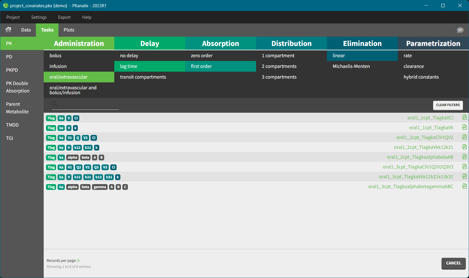
To select a model click on its corresponding line – when all filters are used, only one model is shown. The model will be automatically loaded and displayed in the Model tab. Model filename is displayed on top of the “Model file” section, and has a prefix “lib” to distinguish it from custom models.
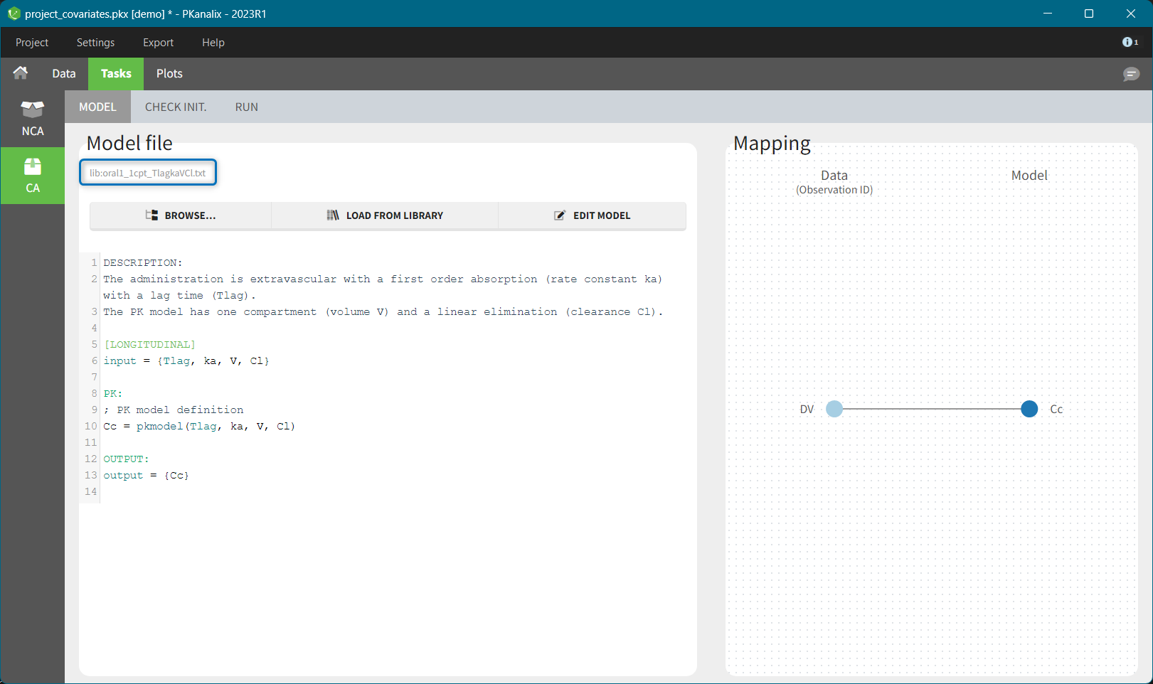
Next section: Custom model
4.1.2.Custom model
In the compartmental analysis task in PKanalix you can use any custom model* – any model written in the Mlxtran language. To load an existing model, click on “BROWSE” in the Model sub tab, and to write a new model from scratch click “NEW MODEL” button.
*Note: In PKanalix versions before 2023, only models from the PK library are available.
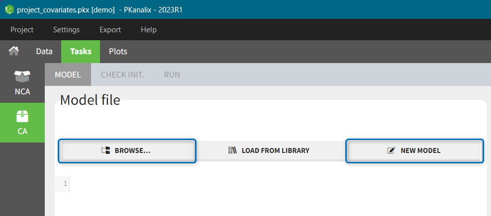
You can also choose a model form the library and then edit it directly in the Model tab by clicking on the button “EDIT MODEL”:
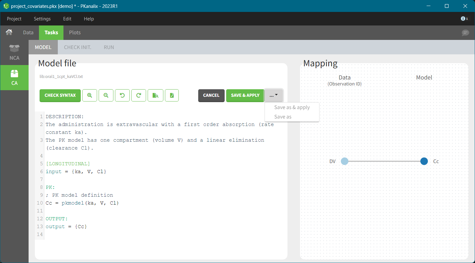
In the edition mode, there are special features that help to write models in mlxtran. It includes functions to color syntax and to detect mlxtran syntax errors, to zoom editing window. In addition, it gives functions and keyword suggestions for the mlxtran language. 
You can save a new model and automatically apply it to a current project – click SAVE & APPLY. To save a model with a different name, use “SAVE AS & APPLY” or “SAVE AS”. Note that models from the library cannot be overwritten.
Merging two models from libraries
In MonolixSuite application there is a dedicated application to write and edit models – mlxEditor. Its functionalities are integrated in the interface, as described above, but you can also use mlxEditor independently of PKanalix. The following video shows an example how to merge two models using mlxEditor.
Writing a model from scratch
The following video describes how to write a custom model. Note that this video uses the old version of mlxEditor, but the functionalities are the same.
Understanding the error messages
The error messages generated when syntax errors occur in the model are very informative and quickly help to get the model right. This video explains the most common error messages..
Next section: Initialization of model parameters
4.2.CA Task
The following page describes how compartmental analysis calculates individual parameters of a model selected in the MODEL tab. Three elements impact this calculation:
- Initialization of model parameters and their constrains on their values
- Cost function used in the optimization algorithm
- Estimation algorithm
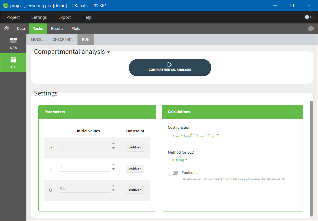
4.2.1.Parameters initialization
Parameters of a model you selected in the MODEL tab are listed in the RUN tab > Settings, see image below. Each parameter has two attributes: an initial value and a constraint.
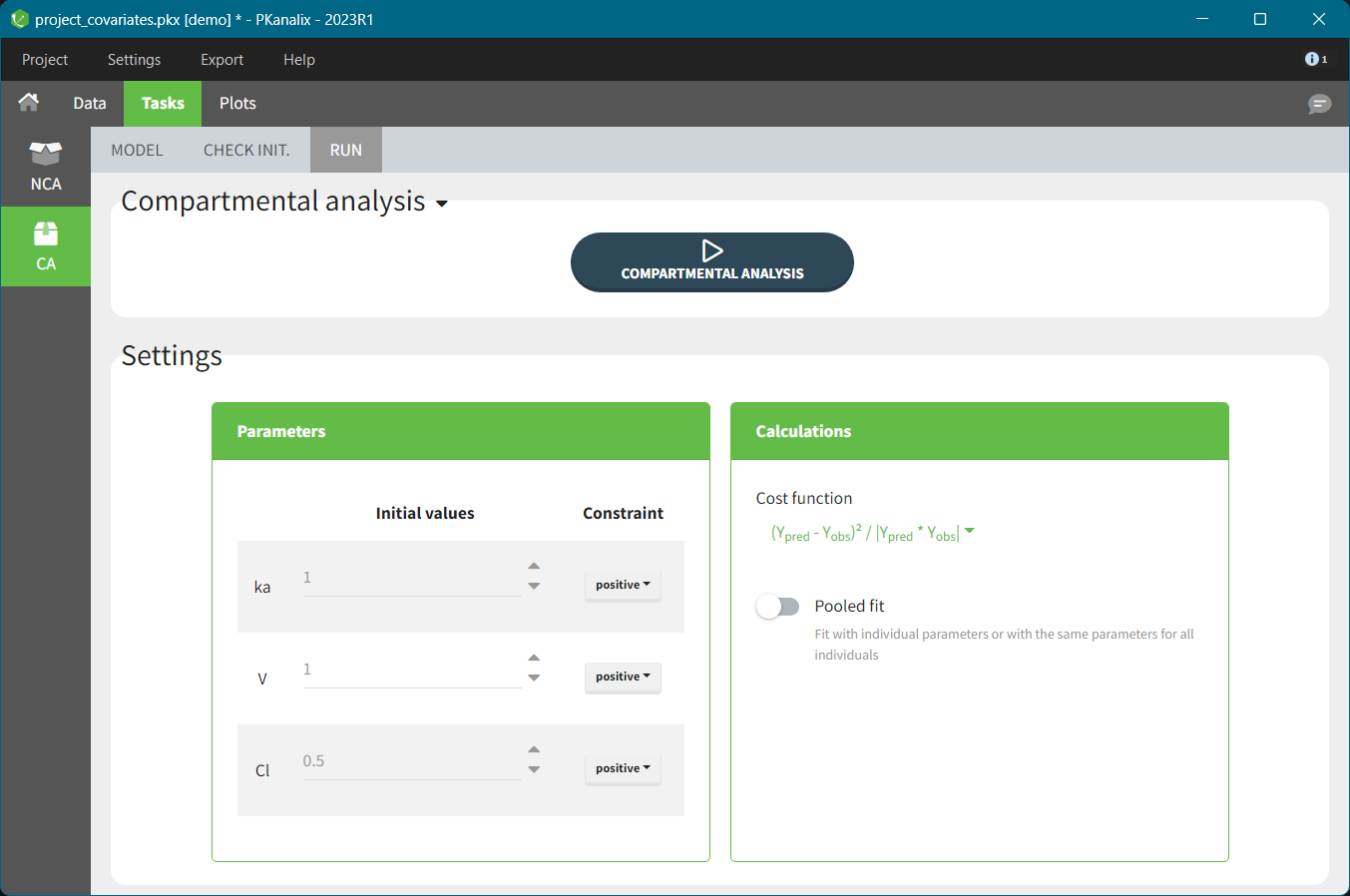
Constraint sets a range of allowed values for selected parameter during estimation (and as initial values). There are three types of constraints:
- none: a parameter is not constraint and its value can be from minus to plus “infinity” (in practice its minus or plus 10e16),
- positive: (default option) a parameter is strictly greater then zero,
- bounded: a parameter is strictly inside a bounded interval which limits you can specify manually.
You can set an initial value of a parameter manually or using the auto-initialization algorithm. Selection of “good” initial values – capturing the characteristic features of a selected model (e.g two slopes on log scale for a 2-compartment model) – is important during the estimation of parameters with the optimization algorithm. It can help to avoid local minima during the optimization process and decrease the runtime of the algorithm.
CHECK INIT.
In the Tasks tab of the CA section there is a dedicated sub-tab CHECK INIT. to help you in the initialization of parameters. The goal of the CHECK INIT. sub tab is to:
- Visually check parameters initialization. It displays the model predictions obtained with the initial model parameters values and the individual designs (doses and regressors) for each individual together with the data points.
- Help finding “good” initial values: manually or with the auto-init function.
CHECK INIT. tab in PKanalix uses the same auto-init algorithm and has the same features as CHECK INIT. in Monolix.
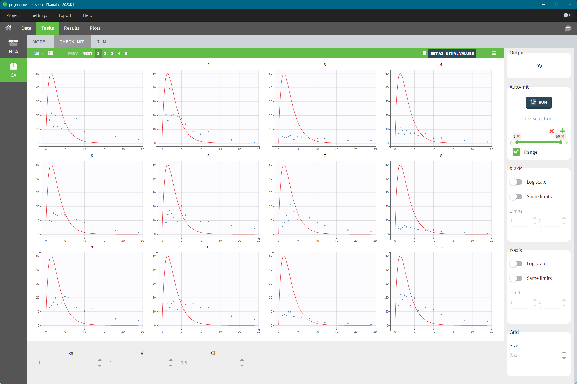
- You can modify the initial values of the parameters, shown on the bottom of the screen, manually by typing new values or using the auto-init algorithm – click the button RUN in the right panel.
- Switch toggle buttons in the X-axis and Y-axis sections to set log-scale and to apply the same limits for all individual plots. It gives a better comparison between the individuals.
- If there are not enough points for the prediction (e.g. there are a lot of doses ), change the grid size by increasing the number of points (last section in the right panel).
IMPORTANT: Click on the “SET AS INITIAL VALUES” button on the top of the plot to save the initial values for the optimization step.
If there are several observation types which obs-ids have been mapped to model outputs (for example a parent and a metabolite, or a PK and a PD observation), then switch the plots between them in the “Output” section on the top-right corner, see figure below.
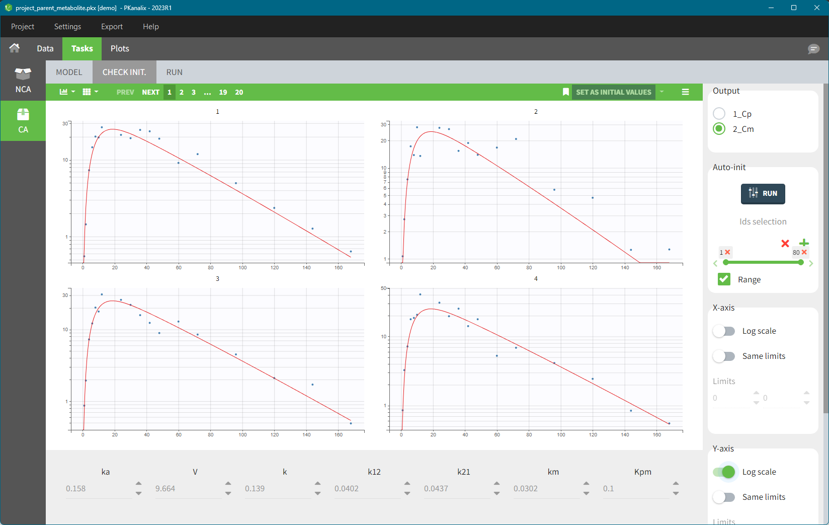
Reference in the “check initial estimates”
The following video describes how to use the Reference option and when it can be helpful. It uses an example in Monolix, but this feature works in the same way in PKanalix.
[/vc_column_text][/vc_column][/vc_row]
Adding a reference helps to see better how changing parameter values impacts the prediction. To add a reference click on the icon next to “Set as initial values” button. It saves the current curve (i.e. current parameters values) as a reference and adds it to the list on top of the right panel, see below. The solid red curve corresponds to the current set of parameters (displayed at the bottom), while the dashed one corresponds to the reference. At any time, you can restore the reference as the current curve (green arrow next to the reference curve name), delete the reference (red cross) or delete all references by clicking on the trash icon above the list.

Auto – init: Automatic initialization of the parameters
PKanalix has an automatic algorithm for the initialization. It is in the right panel in the Auto-init section and you can lunch it by clicking on the button RUN. The following video describes how it works using an example in Monolix.
https://youtu.be/IULGI9Wqahg[
After clicking on the button RUN, PKanalix computes initial model parameters that best fit the data points using a polled fit approach, starting from parameter values currently used in the panel at the bottom. By default, the algorithm uses all individual data from all observations mapped to a model output. You can change the set of individuals in the “Ids” selection panel just below the RUN button.
The algorithm is a custom optimization method, on the pooled data. The purpose is not to find a perfect match but rather to have all the parameters in the good range for starting the Nelder-Mead optimization on each individual.
- While auto-init is running, the pop-up shows the evolution of the cost of the optimization algorithm over the iterations. Stop the algorithm at any time, e.g. if you see that the cost has decreased sufficiently and you want to check the parameter values.
- Note that the more individuals you select, the longer the run will take.
- Selecting one or few individual that show clearly model characteristics (eg a third compartment, a complex absorption) can help the auto-init algorithm to find set of parameters that is sensitive to specific model features.
After running the auto-init, PKanalix interface updates automatically parameter values and plots with new predictions. To use these parameters as initial values in the optimization process, you click on the button “SET AS INITIAL VALUES”.
Note that the auto-init procedure takes into account the current initial values. Sometimes the auto-init might give poor results. To improve it change manually the parameter values before running the auto-init again.
4.2.2.Estimation
The estimation of model parameters is the key function of the compartmental analysis task. In PKanalix it is performed in the framework of generalized least squares estimation. The optimization algorithm consists in minimizing a cost function with an improved version of the Nelder-Mead simplex algorithm, starting from multiple guesses in addition to the initial values provided. To run the algorithm click on the button COMPARTMENTAL ANALYSIS in the RUN tab.
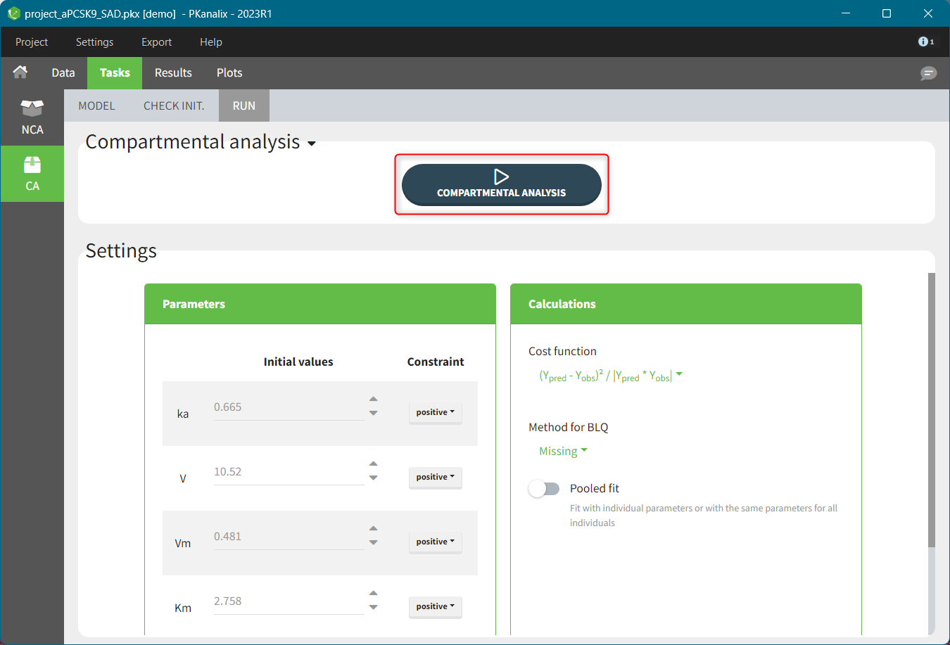
The goal of the optimization is to find model parameters that give the best model fit to the observed data – minimize the objective (cost) function.
- The optimization algorithm performs well in general. However, even if it tries to explore the parameter space, the core algorithm (Nelder-Mead) is local. Therefore proper initialization of parameters is crucial.
- The cost function is described in this documentation page.
- In case of censored data, you can choose a method to treat BLQ data during the optimization: missing, equal to zero, equal to LOQ or equal to LOQ/2.
- By default, the optimization is performed for each individual independently. Switching on the toggle “Pooled fit” in the calculation settings will fit the same parameters to all individuals (data from all individuals is analysed together).
- If occasions are present and pooled fit is not selected, parameters are all considered occasion-dependent so the optimization for every individual includes \( N_{param} \times N_{occ}\) parameters (with \( N_{param} \) the number of parameters in the structural model and \(N_{occ}\) the number of occasions for this individual).
4.2.3.Cost function, AIC and BIC
Cost function and likelihood
Cost function
The cost function that is minimized in the optimization performed during CA is described here. The cost is reported in the result tables after running CA, as individual cost in the table of individual parameters, and as total cost in a separate table, together with the likelihood and additional criteria.
Formulas for the cost function used in PKanalix are derived in the framework of generalized least squares described in the publication Banks, H. T., & Joyner, M. L. (2017). AIC under the framework of least squares estimation. Applied Mathematics Letters, 74, 33-45, with an additional scaling to put the same weight on different observation types.
The total cost function, shown in the COST table in the results, is a sum of individual cost per each occasion (sum over id-occ):
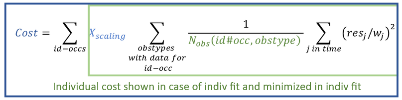
where in the above formula:
- \( N_{obs}(id\#occ, obsType) \) denotes the number of observations for one individual, one occasion and one observation type (ie one model output mapped to data, eg parent and metabolite, or PK and PD, see here).
- \( res_j = Y_{pred}(t_j) – Y_{obs}(t_j) \) are residuals at measurement times \( t_j \), where \(Y_{pred}\) are the predictions for every time point \(t_j\) , and \(Y_{obs}\) the observations read from the dataset.
- \( w_j \) are weights \(1, Y_{obs}, Y_{pred}, \sqrt{|Y_{obs}|}, \sqrt{|Y_{pred}|}, \sqrt{|Y_{obs}|\cdot |Y_{pred}|} \) depending on the choice in the CA task > Settings > Calculations, as explained in this tutorial video.
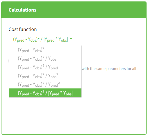
\( X_{scaling} \) is a scaling parameter given by:
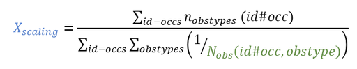
with \( n_{obsTypes}(id\#occ) \) number of observation IDs mapped to a model output for one individual and one occasion. Note that if there is only one observation type (model output mapped to an observation ID), \( X_{scaling} =1\) and the cost function is a simple sum of squares over all observations, weighted by the \(w_j\) .
Likelihood
The likelihood is not directly used for the optimization in CA, but it is possible to derive it based on the optimal cost obtained with the following formula (details in Banks et al):
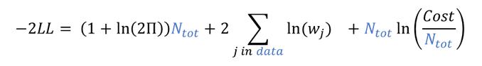
where
- -2LL stands for -2 x ln(Likelihood)
- \( N_{tot} \) is the total number of observations for all individuals, all occasions and all mapped model outputs
- \(w_j\) are the weights as defined above
Additional Criteria
Additional information criteria are the Akaike Information Criteria (AIC) and the Bayesian Information Criteria (BIC). They are used to compare models. They penalize -2LL by the number of model parameters used for the optimization \( N_{param} \), and the number of observations: \( N_{tot} \), total number of observations, and \(N_{obs}(id\#occ)\), number of observations for every subject-occasion. This penalization enables to compare models with different levels of complexity. Indeed, with more parameters, a model can easily give a better fit (lower -2LL), but with too many parameters, a model loses predictive power and confidence in the parameter estimates. If not only the -2LL, but also AIC and BIC criteria decrease after changing a model, it means that the increased likelihood is worth increasing the model complexity.
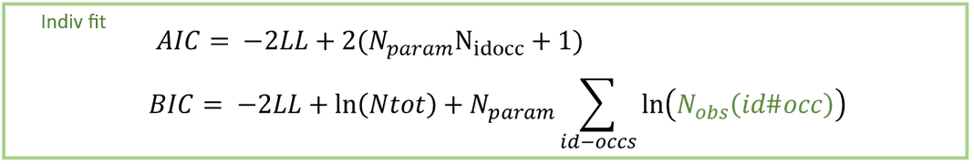
This formula simplifies if the “pooled fit” option is selected in the calculation settings of the CA task:
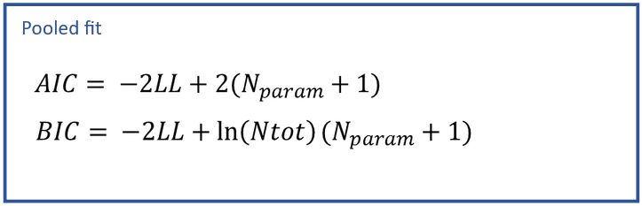
AIC derivation in the case of individual fits
The total AIC for all individuals penalizes -2LL with 2x the number of parameters used in the optimization. For the structural model, we use \(N_{param} N_{id\#occ}\), where \(N_{param}\) is the number of parameters in the structural model and \(N_{id\#occ}\) is the number of subject-occasions (since there is a set of parameters of each id#occ). For the statistical model, we also calculate implicitly one parameter \(\sigma^2\), which is the variance of the residual error model shared by all the individuals (it is derived using the sum of squares of residuals as described in Banks et al). Therefore, AIC penalizes -2LL by \(2(N_{param} N_{idocc} + 1)\).
BIC derivation in the case of individual fits
The total BIC should penalize -2LL by (nb of parameters) x ln(nb of data points). In this case, we should distinguish between the data for each id#occ, which is used to optimize Nparam parameters, and the data for all individuals, which is used all together to calculate the residual variance σ². To penalize each individual’s data in the optimization with Nparam, we add the term \(N_{param} \times ln(N_{obs}(id\#occ))\) for each id#occ. To penalize the calculation of the error model parameter with all the observations (substitution of \(\sigma\) as described in Banks et al), we add the term \(1\times ln(N_{tot})\).
4.3.CA results
PKanalix automatically generates results after running the CA task calculations. This page contains a complete list of output tables and files.
Output tables
Compartmental analysis results are displayed in tables in the “RESULTS” tab, in the CA section.
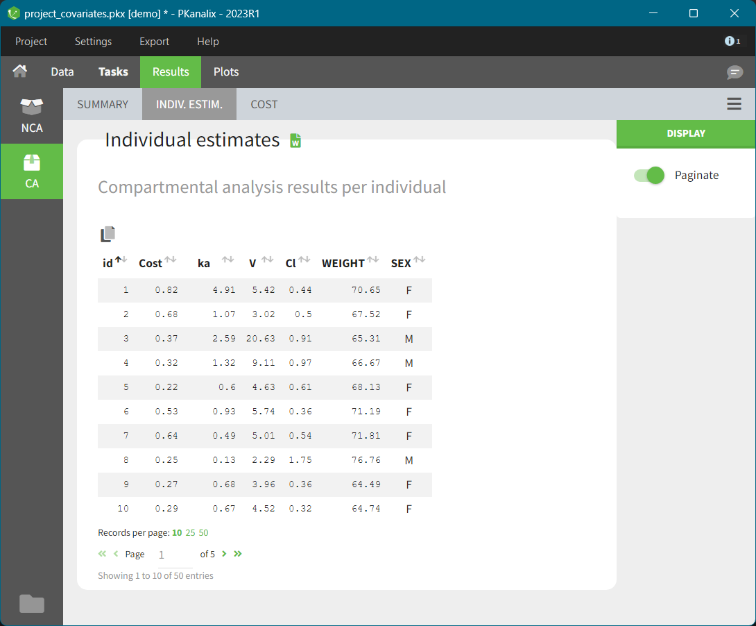
INDIV. ESTIM.
In this table (shown above) you find results of the compartmental analysis for each individual: model parameters values, cost function values, covariates (from the dataset). By default, the table shows 10 records (ids) per page. To increase it and to see following pages, use settings below the table.
SUMMARY
This table contains statistics on compartmental analysis results and summary calculation. The complete list with description is here.
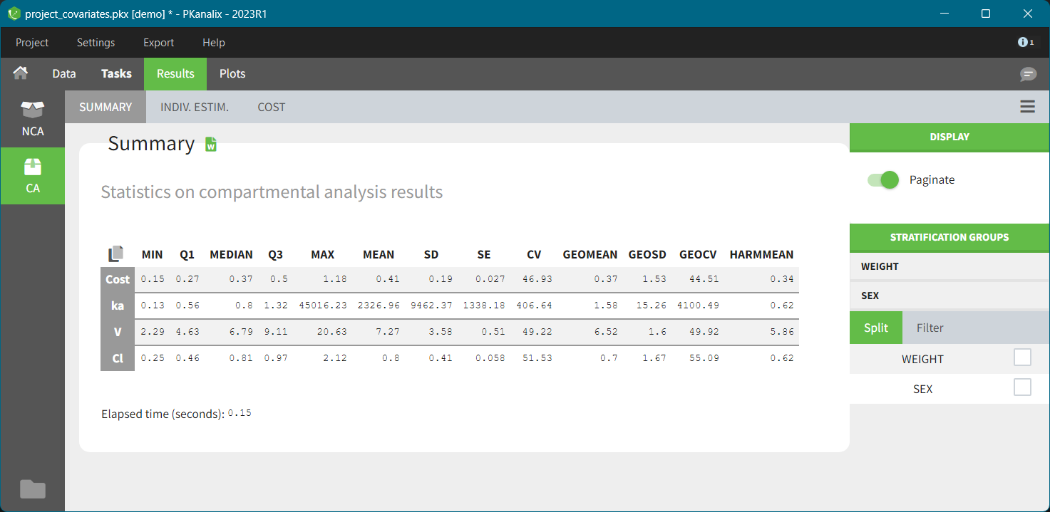
For better comparison you can split or filter this table using covariates present in a dataset. When you select split/filter PKanalix automatically re-calculates the values and displays them. The following Feature of the week video explain how this feature works on the NCA individual estimates table example.
COST
This table contains information about model comparison indices calculated for the model selected in the CA task. It includes: total cost (sum of individual costs values shown in the INDIV. ESTIM. sub tab), -2LL, AIC and BIC, see here for details about the formulas. This information criteria allow to compare statistically the fit obtained with different models. The rule of thumb is: the lower the value of the information criteria, the better the model fit. There is no absolute value to compare with, important is only the relative difference between two models.
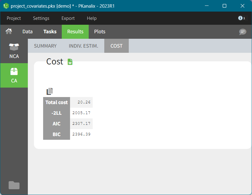
Output Files
You can find the compartmental analysis results also in the project results folder in the “IndividualParameters > ca” directory. There are fours .txt files:
summary.txt
Description: human readable summary file.
Outputs:
- Header: project file name, date and time of run, PKanalix version
- Table: Summary statistics of the individual cost function and individual model parameters
caIndividualParameters.txt
Description: Individual parameters estimates
Outputs:
- ID: subject name and occasion (if applicable). If there is one type of occasion, there will be an additional(s) column(s) defining the occasions.
- Cost: value of the individual cost function
- parameterName: individual model parameter values estimated during the compartmental analysis.
- COVname: continuous covariates values corresponding to all data set columns tagged as “Continuous covariate”.
- CATname: modalities associated to the categorical covariates.
caIndividualParametersSummary.txt
Description: Statistics summary of individual parameters estimates
Outputs:
- ID: subject name and occasion (if applicable). If there is one type of occasion, there will be an additional(s) column(s) defining the occasions.
- Parameter: cost and model parameters
- Statistics: min, Q1, median, Q3, max, mean, SD, SE, CV, geoMean, geoSD, geoCV, harmMean
cost.txt
Description: Total cost and information criteria of a model
Outputs:
- Cost: Total cost, see formulas above
- Log-likelihood estimation: -2LL, AIC, BIC
4.4.Export to Monolix/Simulx
Export a PKanalix to Monolix/Simulx
MonolixSuite applications are interconnected and you can export & import a PKanalix project between different applications. This interconnection is guaranteed by using the same model syntax (mlxtran language) and the same dataset format. There are two options to export a PKanalix project*- Export to Monolix for population model development, estimation and diagnosis. See Monolix documentation.
- Export to Simulx for simulations of new scenarios, e.g. new dosing regimens. It requires loading a model in CA. See Simulx documentation.
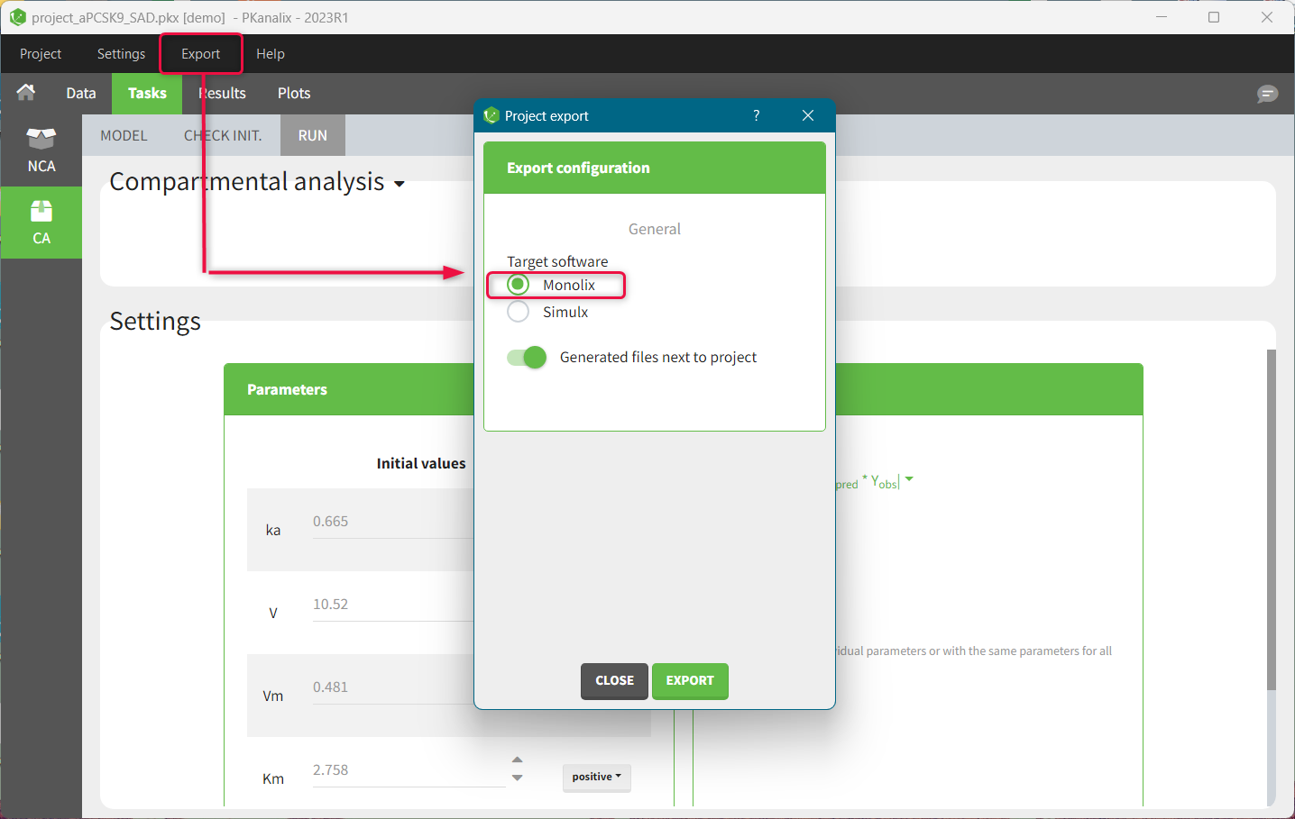
Export to Monolix
Exporting a PKanalix project to Monolix opens automatically a Monolix application and creates a new Monolix project with predefined elements:- Dataset tagging and formatting steps (if present) as in the PKanalix project.
- Dataset filters (if applied) as in the PKanalix project.
- Structural model and initial parameters values as selected in the CA task in the PKanalix project. If there is no model in the PKanalix project, then Monolix will use a default model from the library with oral or iv administration (depending on the NCA settings), one compartment and linear elimination.
- Statistical model and tasks: default Monolix settings
Export to Simulx
Exporting a PKanalix project to Simulx creates a Simulx project with all elements that could be useful for simulating the model automatically. In the Definition tab:- Model, individual parameters estimates and output variables – imported from the CA task in PKanalix.
- Occasions, covariates, treatments and regressors – imported from the dataset used in the PKanalix project.
Share a PKanalix project
The 2024 version of MonolixSuite introduces a highly convenient method for sharing projects. Simply click on “Share Project” in the export menu, and a zip folder is generated containing all the required files to re-open the project (dataset, model for CA if not from library, pkx file, result folder). By default, the suggested location for the zipped shared project matches that of the original, but this can be easily modified to any other location on the computer.5.Bioequivalence
After having run the “NCA” task to calculate the NCA PK parameters, the “Bioequivalence” task can be launched to compare the calculated PK parameters between two groups, usually one receiving the “test” formulation and one the “reference” formulation.
Bioequivalence task
The task “Bioequivalence” is available if at least one categorical covariate column has been tagged in the “Data” tab. The “Bioequivalence” task can only be run after having run the “NCA” task. It can be run by clicking on the “Bioequivalence” task button (pink highlight below) or by selecting it as part of the scenario (tickbox in the upper right corner of the “Bioequivalence” button) and clicking the “Run” button. The parameters to be included in the bioequivalence analysis are selected in the box “Parameters to compute / BE” (orange highlight), where the user can also indicate if the parameter should be log-transformed or not. The fixed effect included in the linear model can be chosen in the box “Bioequivalence design” (blue highlight).
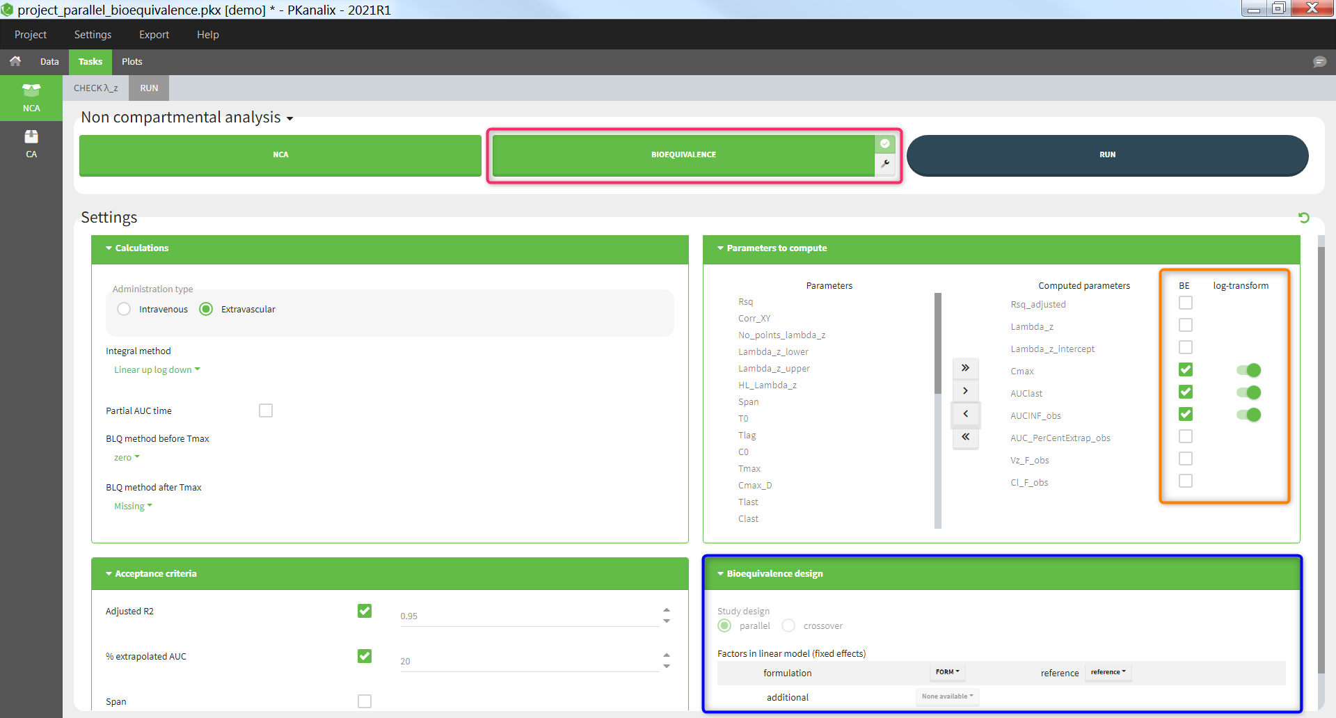
Bioequivalence results
The results of the bioequivalence analysis are presented in the “Results” tab, in the “BE” subtab. Three tables are proposed.
Confidence intervals
The table of confidence intervals is the key bioequivalence table that allows to conclude if the two formulations are equivalent or not. For each parameter selected for bioequivalence analysis, the following information is given:
- the adjusted means (i.e least square means) for each formulation,
- the number of individuals for each formulation,
- the formulation difference (see calculation rules) and the corresponding confidence interval,
- the formulation ratio (see calculation rules) and the corresponding confidence interval.
If N formulations are present in the dataset, N-1 tables are shown.
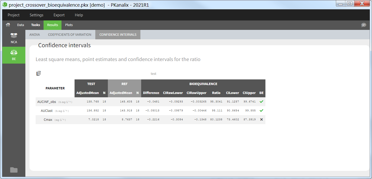
Coefficient of variation
This table gives for each parameter selected for bioequivalence analysis the standard deviation of the residuals and the intra-subject coefficient of variation (CV).
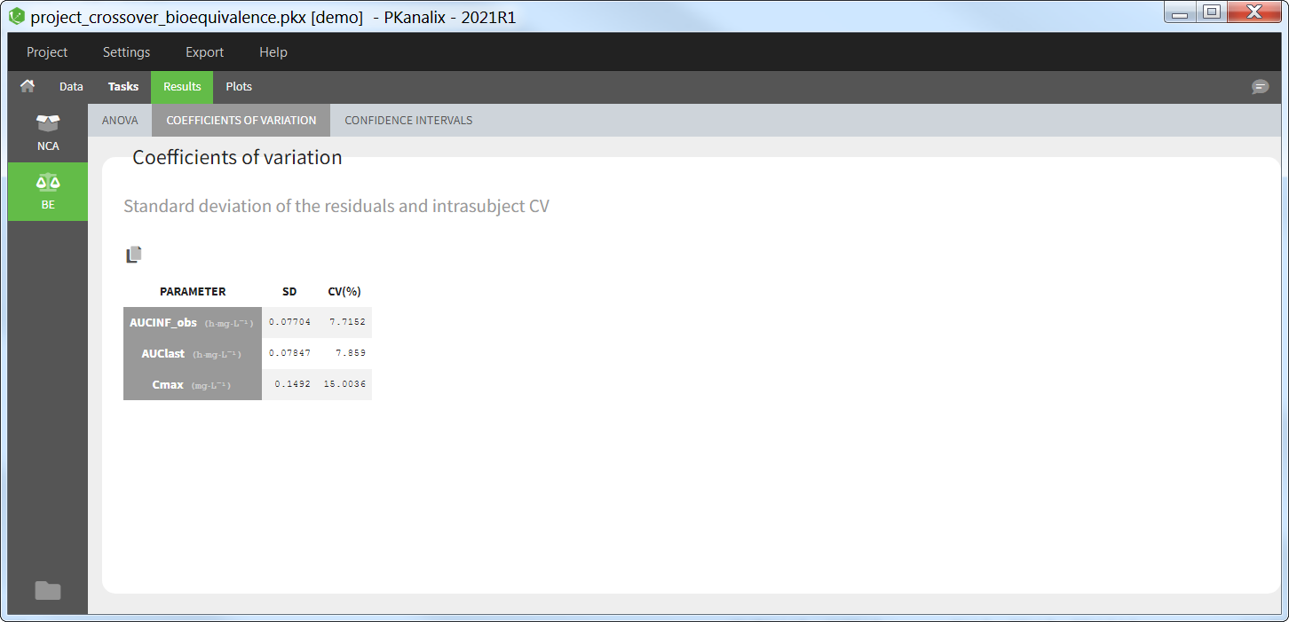
ANOVA
This table presents the analysis of variance (ANOVA) for the factors included in the linear model, for each parameter selected for the bioequivalence analysis. For each factor, the degrees of freedom (DF), sum of squares (SUMSQ), mean squares (MEANSQ), F-value (FVALUE) and the p-value (PR(>F)) are given. A small p-value indicates a significant effect of the corresponding factor.
For the residuals, only the degrees of freedom (DF), sum of squares (SUMSQ), and mean squares (MEANSQ) are given.
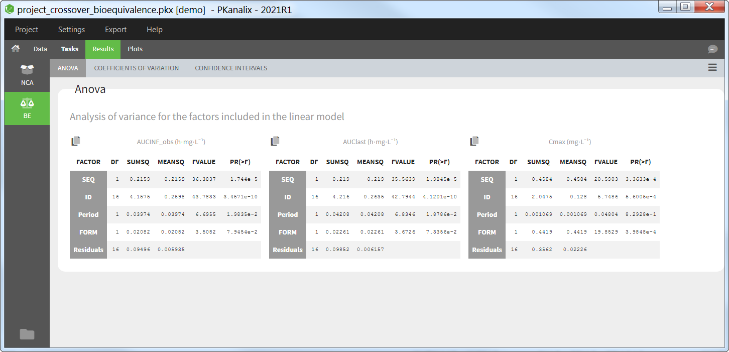
Bioequivalence plots
In the “Plots” tab, several plots are displayed:
- Sequence by period: This plot allows to visualize, for each parameter, the mean and standard deviation for each period, sequence and formulation.
- Subject by formulation: This plot allows to visualize, for each parameter, the subject-by-formulation interaction and the inter-subject variability.
- Confidence intervals: This plot gives a visual representation of the confidence intervals of the ratio of each parameter.
- NCA individual fits: This plot can also be used to display the individual concentration data with one subplot per individual with all its periods.
Bioequivalence outputs
After running the Bioequivalence task, the following files are available in the result folder <result folder>/PKanalix/IndividualParameters/be:
- anova_XXX.txt: these is one such file for each NCA parameter included in the bioequivalence analysis. It contains the ANOVA table with columns ‘Factor’ (factors included in the linear model), ‘Df’ (degrees of freedom), ‘SumSq’ (sum of squares), ‘MeanSq’ (mean squares), ‘FValue’ (F-value), ‘Pr(>F)’ (p-value). For the residuals (last line), the two last columns are empty.
- confidenceInterval_XXX.txt: these is one such file per non-reference formulation. It contains the confidence interval table with columns ‘Parameter’ (parameter name), ‘AdjustedMeanTest’ (adjusted mean for the test formulation), ‘NTest’ (number of individuals for the test formulation), ‘AdjustedMeanRef’ (adjusted mean for the reference formulation), ‘NRef’ (number of individuals for the ref formulation), ‘Difference’ (formulation difference – see calculation rules), ‘CIRawLower’ (lower confidence interval bound for the difference), ‘CIRawUpper’ (upper confidence interval bound for the difference), ‘Ratio’ (formulation ratio – see calculation rules), ‘CILower’ (lower confidence interval bound for the ratio), ‘CIUpper’ (upper confidence interval bound for the ratio), ‘Bioequivalence’ (1 if the CI for the ratio falls within the BE limits, 0 otherwise)
- estimatedCoefficients_XXX.txt: these is one such file for each NCA parameter included in the bioequivalence analysis. It contains the estimated coefficient for each category of each factor included in the linear model, as well as the intercept. This information is only available as an output table and is not displayed in the GUI. The table columns are ‘name’ (factor followed by the category), ‘estimate’ (estimated coefficient), ‘se’ (standard error), ‘tValue’ (estimate divided by the SE), and ‘Pr(>|t|)’ (p-value).
- variationCoef.txt: This file contains the standard deviation and coefficient of variation from each NCA parameter. Columns are ‘Parameter’, ‘SD’ and ‘CV(%)’
5.1.Bioequivalence calculation rules
Detection of “crossover” versus “parallel” design
In PKanalix, the design is detected based on the data set columns. If no OCCASION column is present, the design is detected as “parallel”. On the opposite, if one or several columns have been tagged as OCCASION, the design is detected as “crossover” (repeated or non-repeated). The detected design is displayed in the bioequivalence settings for the users information and cannot be changed. Depending on the detected design, the factors selected by default for the linear model are different.
Linear model
The linear model can only include fixed effects, as recommended by the FDA for parallel and non-repeated crossover design (see Statistical Approaches to Establishing Bioequivalence, page 10) and by the EMA for parallel, non-repeated crossover and repeated crossover designs (see Guideline On The Investigation Of Bioequivalence, page 15). In addition, “id” is automatically considered as nested in “sequence” and no additional nesting can be defined. Interaction terms and random effects are not supported.
According to the regulatory guidelines, the default models are:
- parallel design:
\(\log(\textrm{NCAparam}) \sim \textrm{FORM}\)
which can also be written as
\(\log(\textrm{NCAparam})=\textrm{intercept} + \beta_{test} \textrm{[ if FORM=test]} + \varepsilon\)
in case of two formulations “ref” and “test”, with \(\varepsilon\) a normal random variable (i.e the residuals). - crossover design:
\(\log(\textrm{NCAparam}) \sim \textrm{SEQ + ID + PERIOD + FORM}\)
which can also be written as
\(\log(\textrm{NCAparam})=\textrm{intercept} + \beta_{test} \textrm{[ if FORM=test]} + \beta_{period2} \textrm{[ if PERIOD=2]} + \beta_{seqTR} \textrm{[ if SEQ=TR]} + \beta_{id2} \textrm{[ if ID=id2]} + \beta_{id3} \textrm{[ if ID=id3]} + … + \varepsilon\)
in case of several individuals (id1, id2, etc), two sequences (“RT” and “TR”), two periods (“1” and “2”) and two formulations (“ref” and “test”).
The model parameters are calculated using a QR factorization.
The \(\beta\) parameters are called the coefficients. They are saved in the output file estimatedCoefficients_XXX.txt. We are interested in the coefficient representing the formulation effect \(\beta_{test}\), which is also called the point estimate.
Difference and ratio
In the Results > Confidence intervals table, the “difference” corresponds to the point estimate \(\beta_{test}\) (see above). The “ratio” is calculated depending on the log-transformation choice:
- without log-transformation: \(\textrm{Ratio}=\textrm{LSM}_{test}/\textrm{LSM}_{ref}\times 100\) with \(LSM\) the least square mean (also called adjusted mean, see below).
- with log-transformation: \(\textrm{Ratio}=\exp (\beta_{test}) \times 100\)
Confidence intervals
The confidence interval is first calculated for the difference (\(CI_{diff}\)) and then for the ratio (\(CI_{ratio}\)).
\(CI_{diff}=\beta_{test} \pm t(1-\alpha,df) \times SE \)
with \(\beta_{test}\) the point estimate (“difference”, see above), \(t(1-\alpha,df)\) the quantiles of a Student t-distribution at the \(\alpha\) level and \(df\) degrees of freedom, and \(SE\) the standard error of the point estimate.
In case of a parallel design with the Welch-Satterthwaite correction (see Bioequivalence settings), the formula is different:
\(CI_{diff}=\beta_{test} \pm t(1-\alpha,df) \times \sqrt{\frac{S_R^2}{n_R}+\frac{S_T^2}{n_T}} \)
with \(S_X\) the samples standard deviation of the individuals and \(n_X\) the number of individuals having received formulation X. A correction is also applied to the degrees of freedom, which are calculated as:
\(df=\frac{\left(\frac{S_T^2}{n_T}+\frac{S_R^2}{n_R}\right)^2}{\frac{(S_T^2/n_T)^2}{n_T – 1}+\frac{(S_R^2/n_R)^2}{n_R – 1}}\)
The confidence interval for the ratio is then calculated using the following formula:
- without log-transformation: \(CI_{ratio}=(1+CI_{diff}/\textrm{LSM}_{ref})\times100\) with \(\textrm{LSM}_{ref}\) the least square mean for the reference formulation (see below).
- with log-transformation: \(CI_{ratio}=\exp(CI_{diff})\times 100\)
Adjusted means (least square means)
The model NCAparam ~ SEQ + ID + PERIOD + FORM allows to calculate the expected value (mathematical expectation) for any value of SEQ, ID, PERIOD and FORM. The least square mean for the reference represents the expected value for the reference formulation leaving the value for the other factors undefined. To calculate it, we average the model-predicted values across the levels of ID, PERIOD and SEQ.
The weights assigned to each combination of levels depend if the factors are nested or not. A factor A is said nested in factor B if each level of A appears in only one level of B. By design, in crossover bioequivalence studies, ID is nested in SEQUENCE (i.e each individual belongs to only one sequence). Thus, in PKanalix, when ID and SEQUENCE are defined as factors in the linear model, we assume that ID is nested in SEQUENCE when calculating the least square means. No further nesting is assumed, nor can be specified. Note that the nesting definition only affects the adjusted means and not the point estimate (ratio) and its confidence interval.
Excluded individuals
In case of a parallel design, individuals for which the NCA parameter cannot be calculated are excluded.
In case of a crossover design, incomplete individuals are excluded. Incomplete individual are those that do not have a value for each period, either because these were no concentration data for this period (period missing in the data set) or because the computed NCA parameter could not be calculated for this period (e.g because the data were insufficient to calculate the terminal slope). In case of a non-repeated crossover design, excluding the individuals with missing data or not has no impact on the calculation of the point estimate and confidence interval. In case of a repeated crossover design (i.e when the individuals receive several times the same formulation), excluding the individuals for which the NCA parameter for one or more periods is missing has an impact on the point estimate calculation and confidence interval. The common practice is to exclude incomplete individuals (see also the EMA Guideline On The Investigation Of Bioequivalence, page 14).
Excluded individuals are calculated for each NCA parameter separately, as some individuals may have values for all periods for the Cmax but not the AUCINF_obs for instance.
In the Results > Confidence intervals, the number of individuals “N” does not count the excluded individuals. Thus, in case of a crossover design, the number of individuals contributing to ref and to test is the same. In the BE plots, only the individuals included in the bioequivalence analysis are shown.
ANOVA
The sum of squares presented in the ANOVA table of the Results tab are type-I sequential sum of squares. In case of an unbalanced design (i.e not the same number of individuals receiving RT versus TR), the type-I sum of squares depends on the order of the included factors. In PKanalix, the enforced order is SEQUENCE + ID + PERIOD + FORMULATION (+ ADDITIONAL), following the SAS sample codes provided by the FDA (see Statistical Approaches to Establishing Bioequivalence, 2001, Appendix E) and EMA (see Questions & Answers: positions on specific questions addressed to the Pharmacokinetics Working Party, 2015, question 8).
Coefficient of variation
In Results > Coefficients of variation, the SD corresponds to the standard deviation of the residuals, i.e to the standard deviation of the normal random variable \(\varepsilon\) in the linear model \(\log(\textrm{NCAparam})=\textrm{intercept} + \beta_{test} \textrm{[ if FORM=test]} + \varepsilon\) (for the typical model of a parallel design for instance).
The coefficient of variation is then calculated as:
- without log-transformation: \(CV = SD / LSM_{ref}\) (with \(LSM_{ref}\) the least square mean for the reference formulation, see above)
- with log-transformation: \(CV = 100 \times \sqrt{\exp{(SD^2)}-1}\)
5.2.Bioequivalence settings
This page describes the settings of the bioequivalence calculations.
Parameters to compute
In the section “Parameters to compute”, the user can move the parameters from the “Parameters” column (list of all available parameters) to the “Computed parameters” column to select them for the NCA calculations. Among the parameters selected for the NCA calculations, the user can choose which parameters should be included in the bioequivalence analysis by ticking the box in the “BE” column. Regulatory guidelines usually recommend to perform the bioequivalence on the log-transformed NCA parameters. This can be set using the toggles in the “log-transform” column.
- BE: parameters on which to perform the bioequivalence analysis. Defaults: Cmax, AUClast, and AUCINF_obs if plasma single-dose, or AUCtau and Cmax if plasma steady-state, or AURC_last and Max_Rate if urine data.
- log-transform: whether the bioequivalence should be computed on the log-transformed NCA parameter (toggle on) or on the NCA parameter directly (toggle off). Default: log-transform toggle on, except for Tmax.
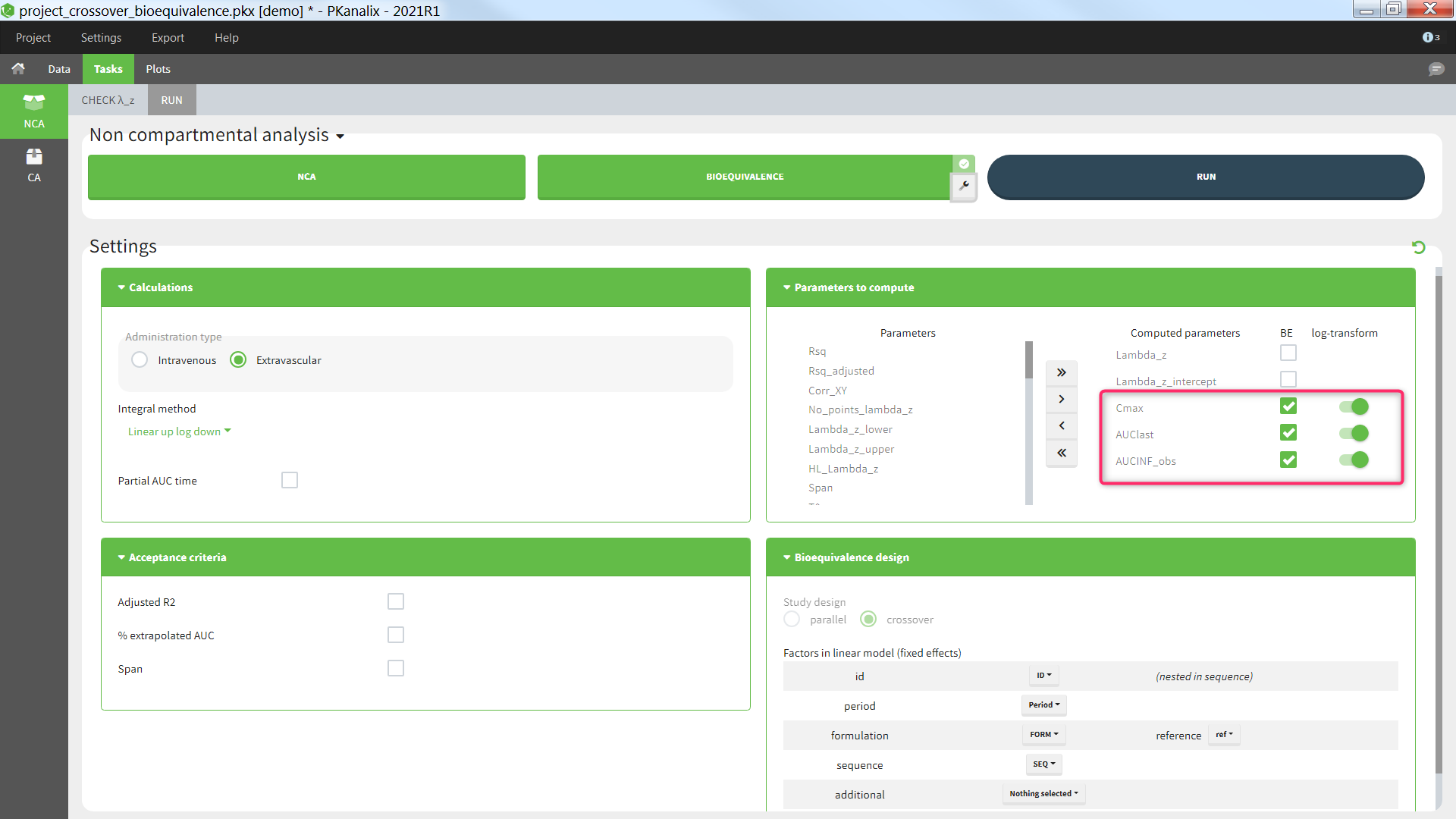
Bioequivalence design
The study design, parallel or crossover (repeated or not), is detected automatically based on the structure of the ID and OCCASION columns of the data set, see the Calculation rules for more details. The user can then select one or several fixed effect factors to be included in the linear model. By default, for a parallel design, only the formulation is included. For a crossover design, the factors ID, PERIOD, FORMULATION and SEQUENCE are included by default, if present in the data set. When both ID and SEQUENCE are given, ID is considered as nested in SEQUENCE. Additional factors can also be added, to be chosen among the (STRATIFICATION) CATEGORICAL and CONTINUOUS COVARIATES columns of the data set. All factors are considered as fixed effects and random effects are not available. Nesting of ID in SEQUENCE is considered automatically, but further nesting cannot be specified. Note that the nesting affects the calculation of the adjusted means but not of the bioequivalence ratio.
- Study design: parallel or crossover (repeated or not-repeated). Detected automatically based on the structure of the ID and OCCASION columns of the data set (see Calculation rules). Cannot be changed by the user.
- Factors in the linear model:
- id [if crossover]: data set column representing the ID of the individuals. Default: the column tagged as ID in the data set. This can be set to “none” if the ID should not be used as a factor in the linear model. When a “sequence” column is defined, “id” is considered as nested in “sequence”.
- period [if crossover]: data set column representing the different periods for each individual. Default: the first column tagged as OCCASION in the data set. This setting can be set to “none” if the period should not be used as a factor in the linear model.
- formulation: data set column representing the different groups for which the bioequivalence is calculated, typically the different formulations of the drug products. Default: the column with header ‘trt’, ‘treatment’, ‘form’, or ‘formulation’ (case insensitive) if it exists, otherwise first CATEGORICAL COVARIATE column. It is mandatory to include the formulation in the linear model.
- reference: among the categories of the categorical covariate selected as formulation, the one considered as the reference. The bioequivalence will be computed for all categories compared to the reference category. Default: ‘r’ or ‘ref’ or ‘reference’ (case insensitive), otherwise the category of the first occasion of the first indiv of the data set.
- sequence [if crossover]: data set column representing the different sequences. Default: the column with header ‘seq’, or ‘sequence’ (case insensitive) if it exist, otherwise “none”. This setting can be set to “none” if the sequence should not be used as a factor in the linear model.
- additional: data set columns tagged as CATEGORICAL or CONTINUOUS covariates, which have not already been selected above, can be added as additional factors in the linear model.
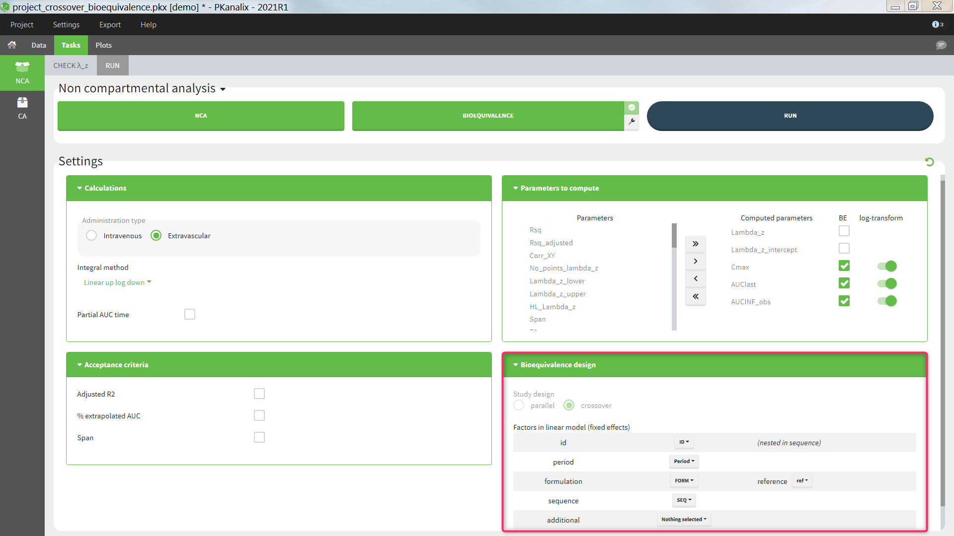
Confidence interval
Several settings are more specific to the calculation of the confidence interval. They can be changed in the pop-up settings window of the Bioequivalence task.
- Level: level of the confidence interval. Default: 90% confidence interval. This means that there is a 90% probability that the true ratio is included in the calculated confidence interval.
- Bioequivalence limits: limits within which the confidence interval should be in order to conclude for bioequivalence. Default: [80,125].
- Degrees of freedom [if parallel design]: method to calculate the degrees of freedom involved in the confidence interval calculations, either using the residuals (this assumes equal variance between the groups or using the Welch-Satterthwaite formula (this assumes possibly unequal variances). Default: Welch-Satterthwaite
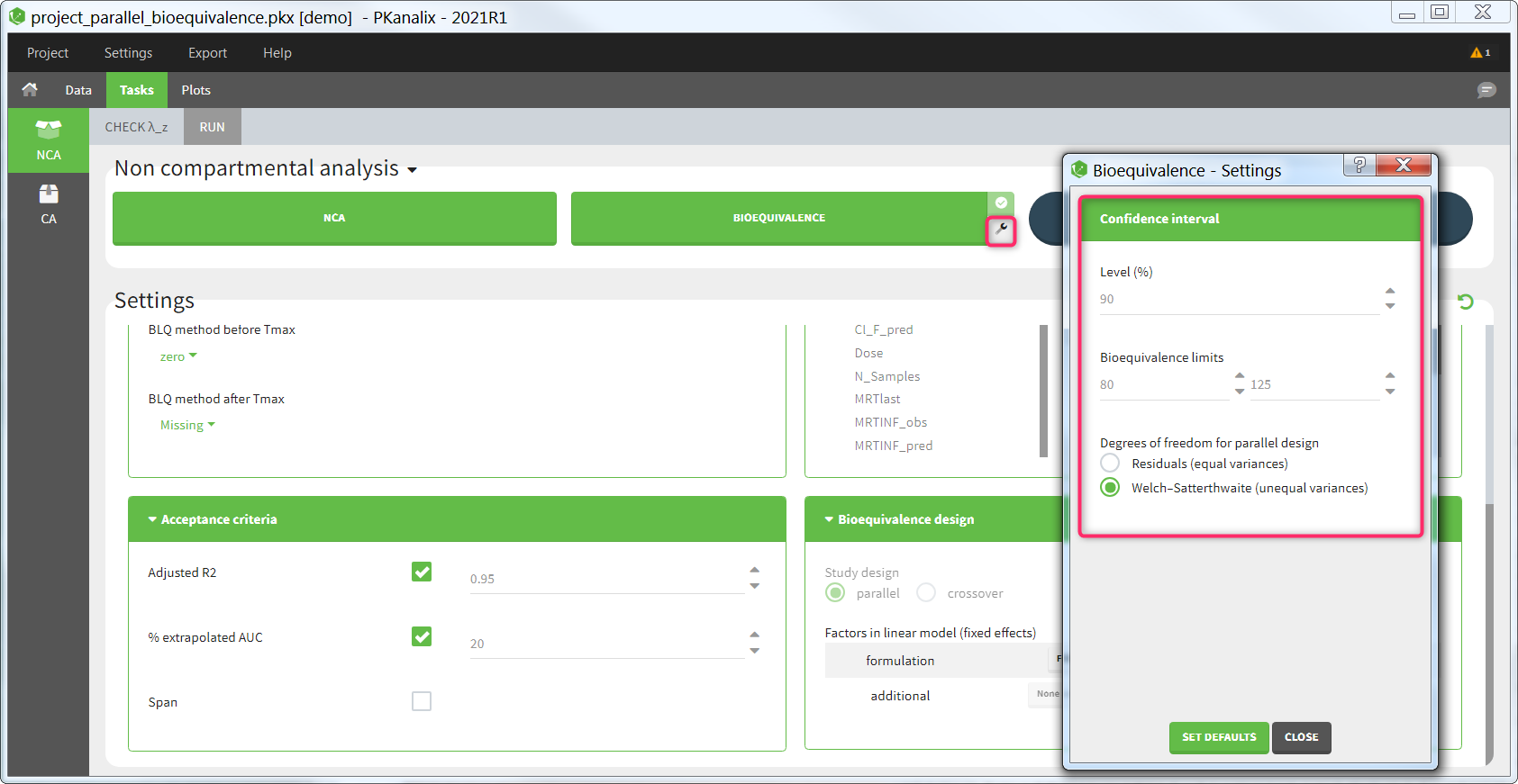
6.Plots
For the CA task, PKanalix generates automatically specific plots to help in model diagnosis. Plots are interactive for better data exploration. You can modify display options (lin/log scales, axis limits, etc), stratify (split, color, filter) them using covariates from a dataset, and change the graphical preferences (font size, colors etc).
In the PLOTS tab you will find the following plots:
- Individual fits This plot displays the individual predictions using the individual estimated parameters (or one set of common parameters if you enable the “pooled fit” option) w.r.t. time on a continuous grid, with the observed data overlaid.
- Individual parameters vs covariates This plot displays estimated individual parameters w.r.t. the covariates in the dataset.
- Distribution of the individual parameters. This plot displays the estimated population distributions of the individual parameters.
- Correlation between individual parameters This plot displays scatter plots for each pair of individual parameters.
- Observations vs predictions This plot displays observations w.r.t. the predictions computed using the individual parameters (or one set of common parameters if you enable the “pooled fit” option).
Stratification & Preferences
Stratification of plots in PKanalix works in the same way as in Monolix. Complete description of available options and examples is in the Monolix documentation here.
Save/Export plots and charts data
You can export each single plot as an image (png or svg) using an icon on top of each plot. They are saved in the results folder > PKanalix > ChartsFigures.
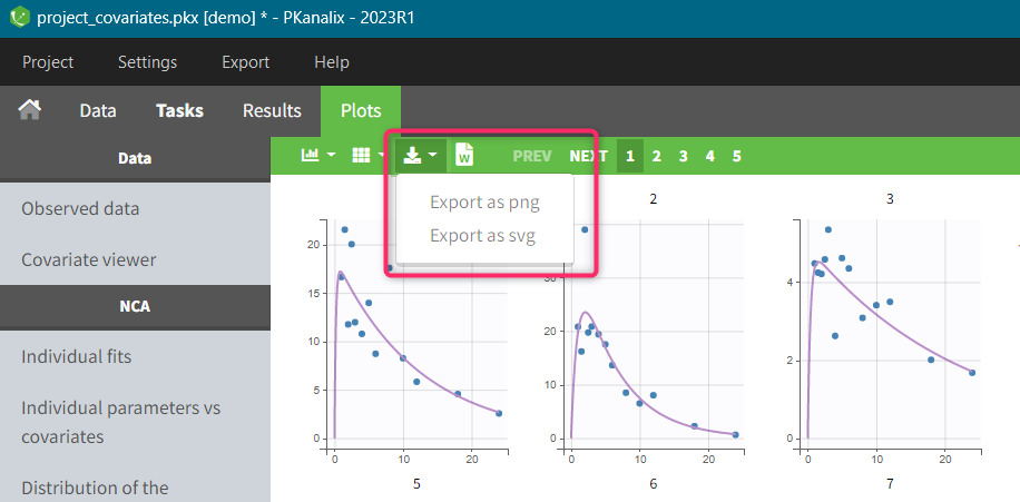
To export all plots at once use the top menu option: “Export > Export Plots”. You can also export plots data as tables (in .txt files), for example to re-generate them with external tools, with “Export > Export charts data”.
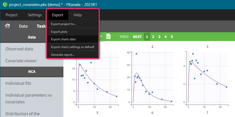
In addition, you can export plots automatically after each CA run. To select this option enable the toggle buttons in the PKanalix Preferences: top menu > Settings > Preferences:
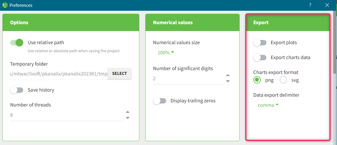
Next section: CA Individual fits plot
6.1.Data
6.1.1.Observed data
The purpose of this plot, also called a spaghetti plot, is to display the original data w.r.t. time.
In the example below, the concentration of warfarin from the warfarin data set is displayed. A subject is highlighted in yellow by hovering on the line.
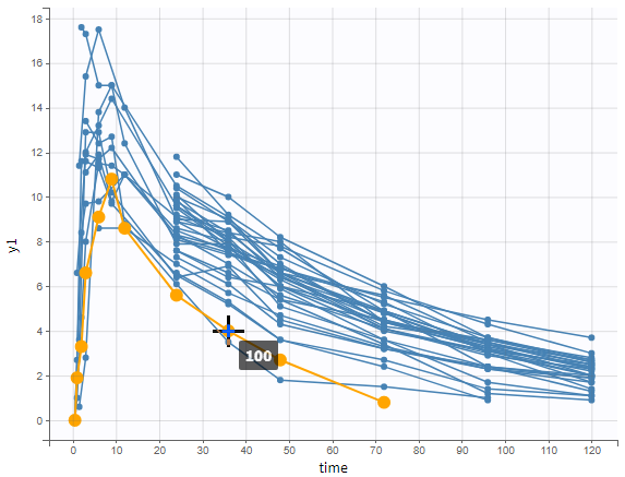 One can plot the output in a log-scale to have a better evaluation of the elimination part for example as in the figure below.
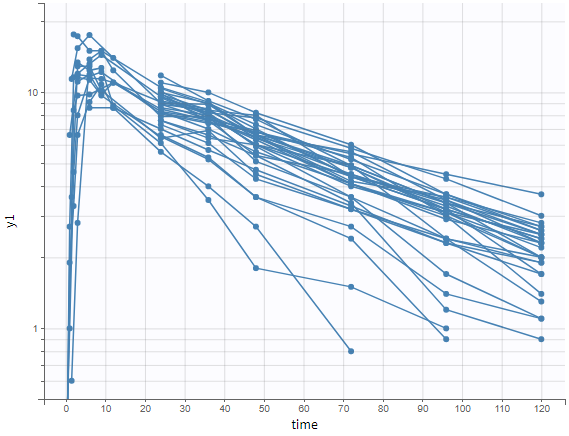
The data can be displayed as dots and lines (by default), or only as dots or only as lines, as in the figure below. In addition, a trend line can be overlaid on the plot, based on mean values of the observed data pooled in bins. The user can choose arithmetic or geometric mean, and can add error bars representing either the standard deviations or standard errors. The mean and error values can be displayed as fixed labels next to the bars, or as tooltips when hovering on a bar.
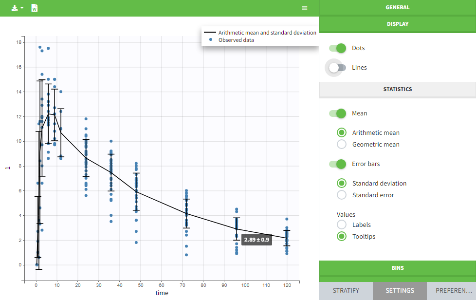
Bin limits can be displayed as vertical lines, and the user can change the number of bins as well as binning criteria.
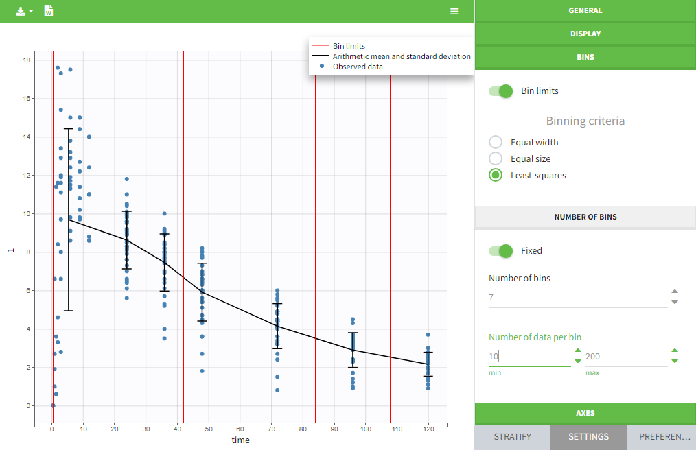
An interesting feature is the possibility to display the dosing time as on the figure below. The individual dosing time of the individual can be displayed when the user hovers an individual or always visible. Starting in version 2021R1 on, dosing times corresponding to doses with null amounts are not displayed.
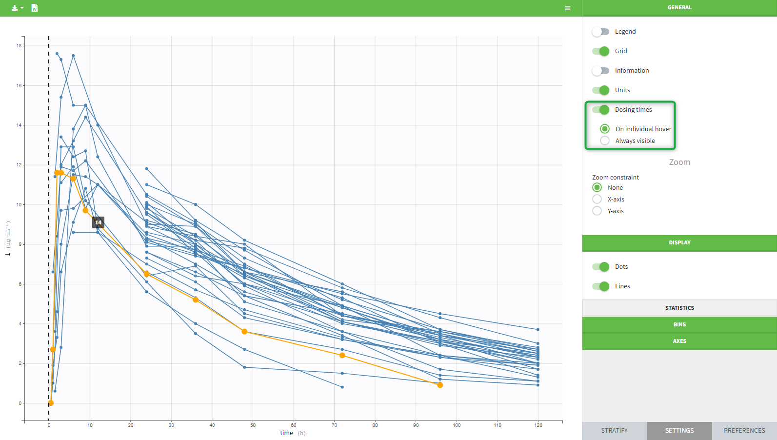
The units as well as additional descriptive statistics of the observations can be displayed. We propose
- The total number of subjects
- The average number of doses per subject
- The total, average, minimum and maximum number of observations per individual.
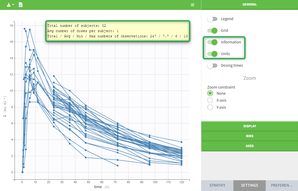
In addition, if we split the graphic with a covariate, these numbers are recomputed to display the information of the group as in the following plot.
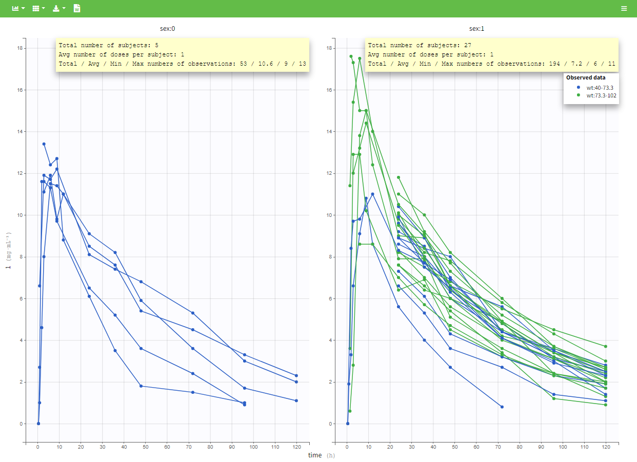
In PKanalix 2023R1 it is now possible to display the mean curves, split by covariate, in a single plot. By switching on the “Merged splits” option, the mean curves of the two wiehgt groups, which appeared in previous versions in separate plots, are merged into a single plot.
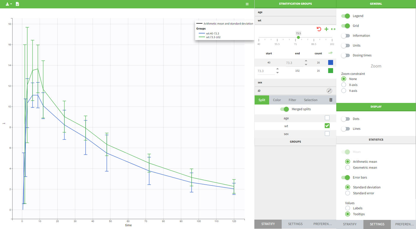
6.1.2.Covariate viewer
It is possible to show the matrix of all the covariates as on the following figure:
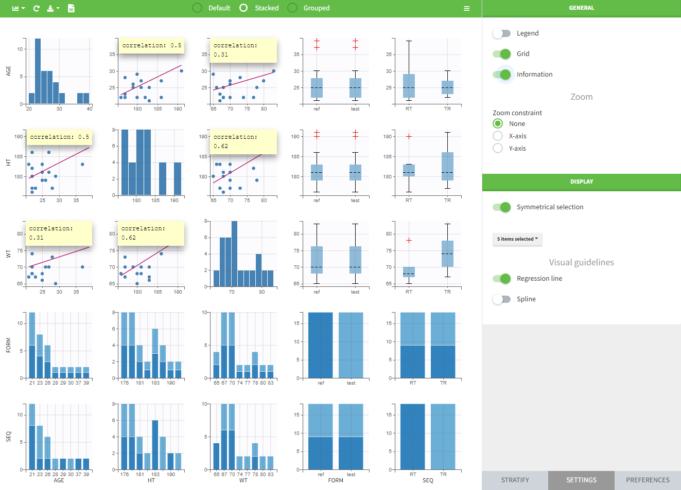
It is possible to display one covariate vs another one, selecting in the display panel which covariate to look at.
Here we display the weight versus the height and show the correlation coefficient as an information:

Categorical covariates w.r.t. other categorical covariates are displayed as a histogram (stacked or grouped),

and continuous covariates w.r.t. categorical covariates are displayed as a boxplot as below (“+” are outlier points below Q1-1.5IQR (interquartile range) or above Q3+1.5IQR):

Covariate statistics
Starting from the 2021 version, it is also possible to get the covariate statistics in a dedicated frame of the interface:
All the covariates (if any) are displayed and a summary of the statistics is proposed. For continuous covariates, minimum, median and maximum values are proposed along with the first and third quartile, and the standard deviation. For categorical covariates, all the modalities are displayed along with the number of each. Note the “Copy table” button that allows to copy the table in Word and Excel. The format and the display of the table will be preserved.
6.1.3.Bivariate data viewer
In case of several continuous outputs, one can plot one type of observation w.r.t. another one as on the following figure for the warfarin data set. The direction of time is indicated by the red arrow. Linear interpolation is used for observations of different types that are not at the same time.
Labels for x and y axes correspond to the observation names in the model for data types that are mapped to an output of the model, or observation ids used in the dataset for data types not captured by the model. It is possible to choose which observation id to display on the X or Y axis in the settings panel on the right.
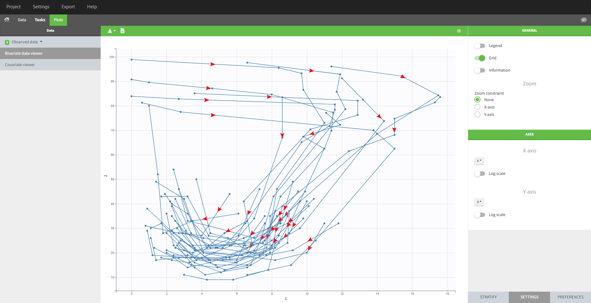
6.2.NCA
6.2.1.NCA individual fits
Purpose
This plot can be used for two purposes:
- show the terminal slope (lambdaZ) linear regression for each occasion of each individual (default)
- show the individual concentration data with one individual per subplot and all occasions
LambdaZ terminal slope
By default, the settings let you see each occasion of each individual on a subplot, in y log-scale with the lambdaZ linear regression. Note that the NCA parameters Lambda_z and Lambda_z_intercept need to be selected in the “Computed parameters” of NCA settings in order to display the lambdaZ regression line.
Selecting the “Information” toggle allows you to display information about the rule used to calculated the lambdaZ (“Adjusted R2”, “R2”, “Interval”, “Points” or “custom” – when points have been manually selected), the number of points included in the calculation and the R2 or adjusted R2 criteria. Again, the NCA parameters Rsq_adjusted, Rsq, and No_points_lambda_z must be selected in “Computed parameters” in the NCA settings in order to appear in the information box.
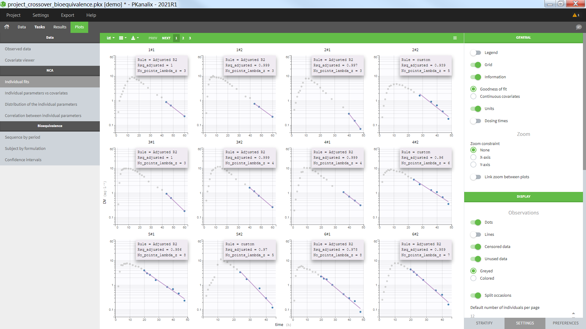
Individual concentration data
The plot can also be used to visualize the individual concentration data with one individual per subplot and occasions all together. For a crossover study with two periods and two formulations for instance, one can:
- display the “Lines”
- display the “unused data” as “colored”
- hide the “LambdaZ regression”
- untick the “split occasions”
- set the y axis in linear scale
- color by the Formulation in the stratify tab
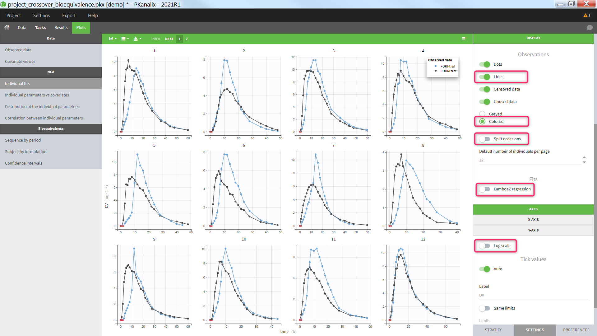
Settings
- Grid arrange (top left above the plot): The user can define the number of subplots displayed, as well as the number of rows and the number of columns. This choice is not saved. See below the “Default number of individuals per page” for a setting that is saved.
- General
- Legend: hide/show the legend. The legends adapts automatically to the elements displayed on the plot. The same legend box applies to all subplots and it is possible to drag and drop the legend at the desired place.
- Grid : hide/show the grid in the background of the plots.
- Information: hide/show
- the continuous covariates: continuous covariates values are displayed for each individual
- the goodness of fit: the rule used to calculate the lambdaZ (“Adjusted R2”, “R2”, “Interval”, “Points” or “custom” – when points have been manually selected), the number of points used to calculate the lambdaZ and the R2 value (if rule=R2) or the adjusted R2 (if rule different from R2). Note that the NCA parameters Rsq_adjusted, Rsq, and No_points_lambda_z must be selected as “Computed parameters” in the NCA settings in order to appear in the information box.
- Units: hide/show the units next to the NCA parameter names. The color and surrounding characters for the units can be chosen in the plot “Preferences”.
- Dosing times: hide/show dosing times as vertical lines for each subject.
- Link zoom between plots: activate the linked zoom for all subplots. The same zooming region can be applied on all individuals only on the x-axis, only on the Y-axis or on both (option “none” in the “zoom constraint”).
- Display
- Dots: hide/show the observed data as dots
- Lines: hide/show the connecting lines between the observed data points
- Censored data [if censored data present]: hide/show the data marked as censored (BLQ), shown as a red dot according to the “BLQ method before/after Tmax” choice in the NCA settings.
- Unused data: hide/show the data points not used for the lambdaZ calculation
- greyed: display the data points not used in the lambdaZ calculation as greyed
- colored: display the data points not used in the lambdaZ calculation with the default color (set in the plot “Preferences”)
- Split occasions [if occasions present]: Split the individual subplots by occasions or group occasions on a single subplot for each individual.
- Default number of individuals per page: Set the number of subplots to display. This setting can be saved, whereas the “grid arrange” on the top left corner is not.
- LambdaZ regression: hide/show the lambdaZ linear regression
- Sorting: Sort the subjects by ID, goodness of fit (R2 or adjusted R2 value) or continuous covariate value in ascending or descending order.
6.2.2.Distribution of the NCA parameters
Purpose
This figure can be used to see the empirical distribution of the NCA parameters. Further analysis such as stratification by covariate can be performed and will be detailed below.
PDF and CDF
It is possible to display the theoretical distribution and the histogram of the empirical distribution as proposed below.
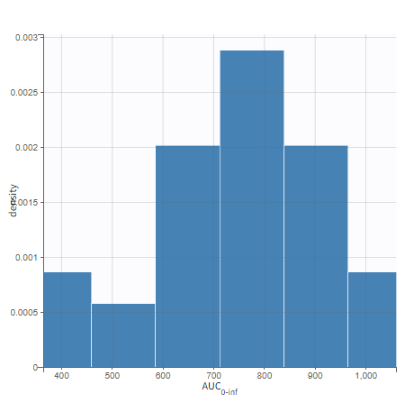
The distributions are represented as histograms for the probability density function (PDF). Hovering on the histogram also reveals the density value of each bin as shown on the figure below

Cumulative distribution functions (CDF) is proposed too.
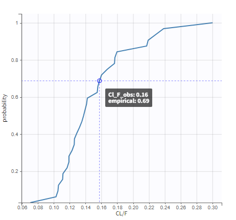 Example of stratification
It is possible to stratify the population by some covariate values and obtain the distributions of the individual parameters in each group. This can be useful to check covariate effect, in particular when the distribution of a parameter exhibits two or more peaks for the whole population. On the following example, the distribution of the parameter k from the same example as above has been split for two groups of individuals according to the value of the sex, allowing to visualize two clearly different distributions.
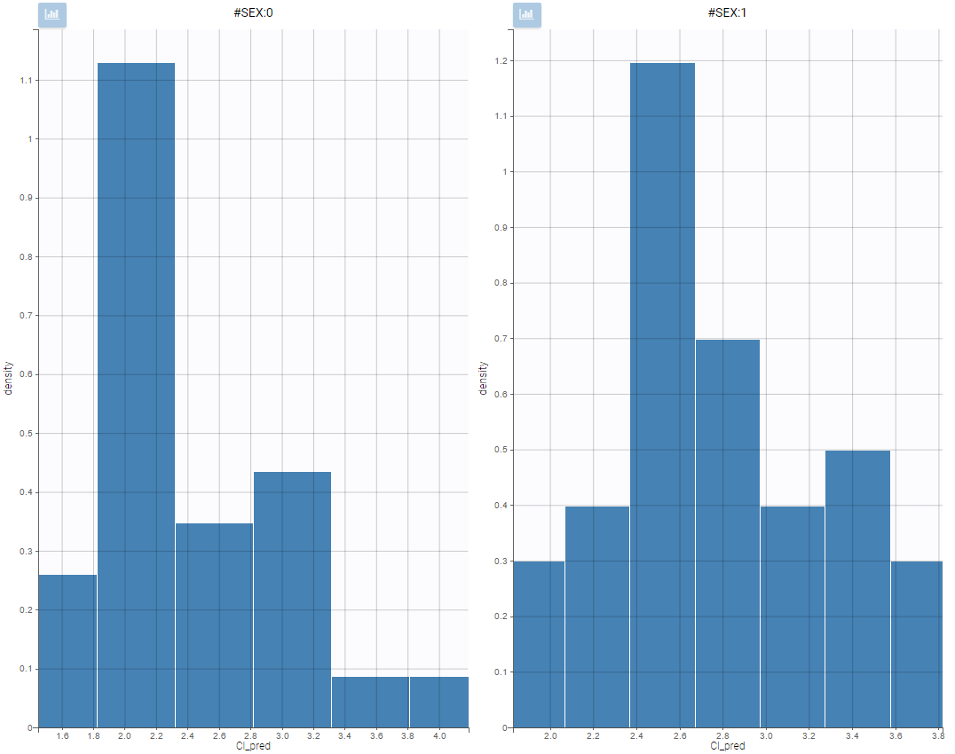 Settings
- General: add/remove the legend, and the grid
- Display
- Distribution function: The user can choose to display either the probability density function (PDF) as histogram or the cumulative distribution function (CDF).
6.2.3.NCA parameters with respect to covariates
Purpose
The figure displays the individual parameters as a function of the covariates. It allows to identify correlation effects between the individual parameters and the covariates.
Identifying correlation effects
In the example below, we can see the parameters Cl_obs and Cmax with respect to the covariates: the weight WT, the age AGE and the sex category.
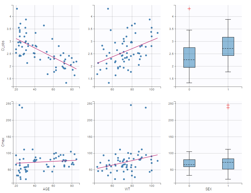
Visual guidelines
In order to help identifying correlations, regression lines, spline interpolations and correlation coefficients can be overlaid on the plots for continuous covariates. Here we can see a strong correlation between the parameter Cl_obs and the age and the weight.
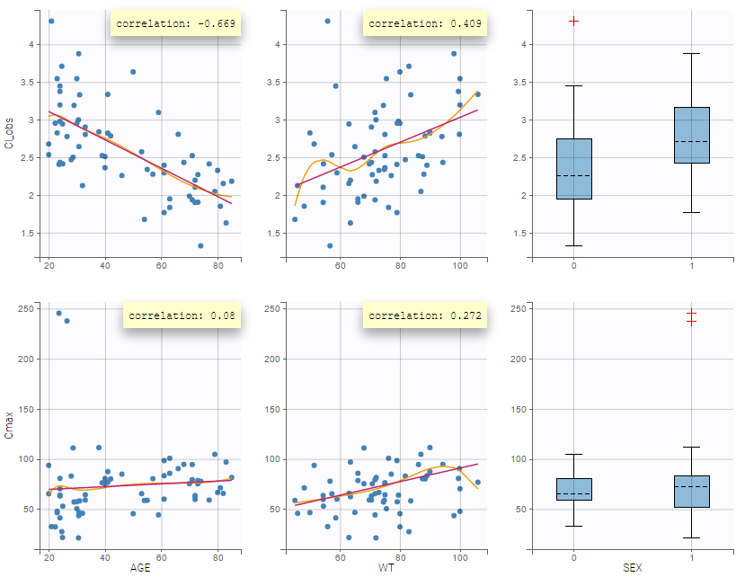
Overlay of values on top of the boxplot
The NCA parameter values used to generate the boxplots for the categorical covariates can be overlayed on top of the boxplots, which enables to better visualize the distribution in case of a small number of individuals.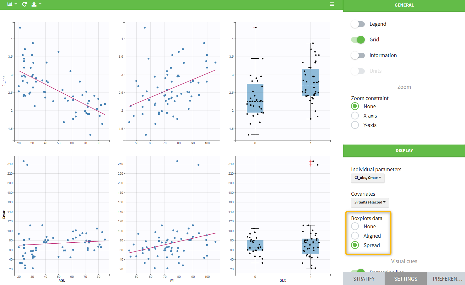
Highlight
Hovering on a point reveals the corresponding individual and, if multiple individual parameters have been simulated from the conditional distribution for each individual, highlights all the points points from the same individual. This is useful to identify possible outliers and subsequently check their behavior in the observed data.
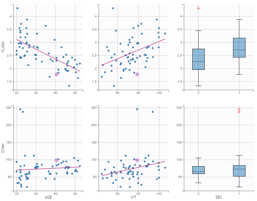
Selection
It is possible to select a subset of covariates or parameters, as shown below. In the selection panel, tick the items you would like to see and click “Accept”. This is useful when there are many parameters or covariates. 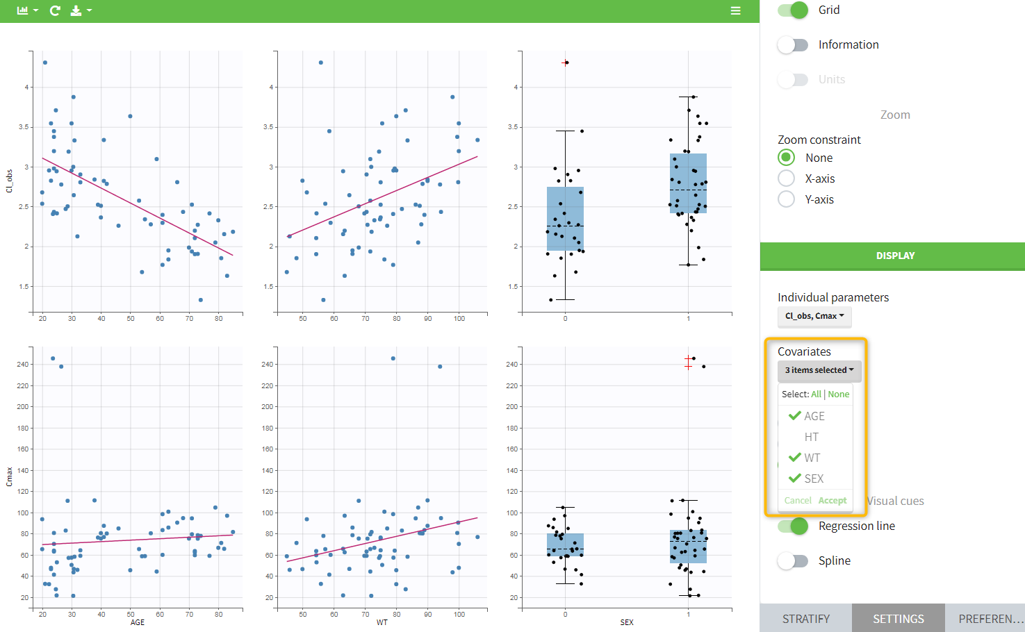
Stratification
Stratification can be applied by creating groups of covariate values. As can be seen below, these groups can then be split, colored or filtered, allowing to check the effect of the covariate on the correlation between two parameters. The correlation coefficient is updated according to the split or filtering.
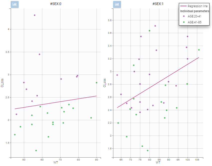
Settings
- General
- Legend: add/remove the legend. There is only one legend for all plots.
- Grid: add/remove the grid.
- Information: display/hide the correlation coefficient associated with each scatter plot.
- Units: display/hide the units of the NCA parameters on the y axis
- Display
- Individual parameters: Selects the NCA parameters to display as subplot on rows. Tick the items you would like to see and click “accept”.
- Covariates: Selects the NCA parameters to display as subplot on columns. Tick the items you would like to see and click “accept”.
- Boxplots data: overlay the NCA parameters as dots on top of the boxplots for categorical covariates, either aligned on a vertical line (“aligned”), spread over the boxplot width (“spread”) or not at all (“none”).
- Regression line: Add/remove the linear regression line corresponding to the correlation coefficient.
- Spline: Add/remove the spline. Spline settings cannot be changed.
6.2.4.Correlation between NCA parameters
Purpose
This plot displays scatter plots for each pair of parameters. It allows to identify correlations between parameters, which can be used to see the results of your analysis and see the coherence of the parameters for each individuals.
Example
In the following example, one can see pairs of parameters estimated for all parameters.

Visual guidelines
In addition to regression lines, correlation coefficients can been added to see the correlation between random effects, as well as spline interpolations.
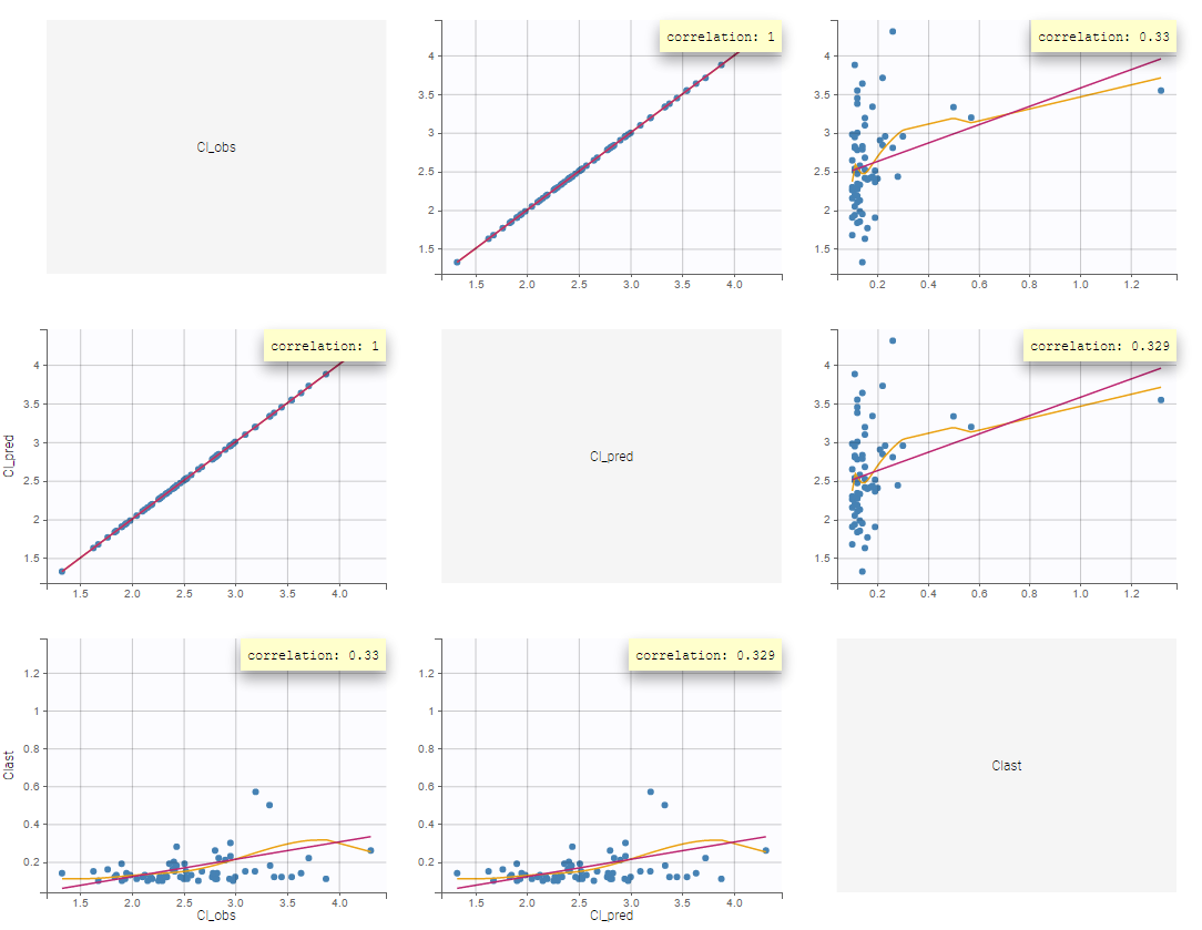
Selection
It is possible to select a subset of parameters, whose pairs of correlations are then displayed, as shown below. In the selection panel, a set of contiguous rows can be selected with a single extended click, or a set of non-contiguous rows can be selected with several clicks while holding the Ctrl key.
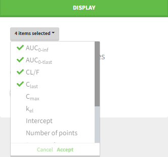
Highlight
Similarly to other plots, hovering on a point provides information on the corresponding subject id, and highlights other points corresponding to the same individual.
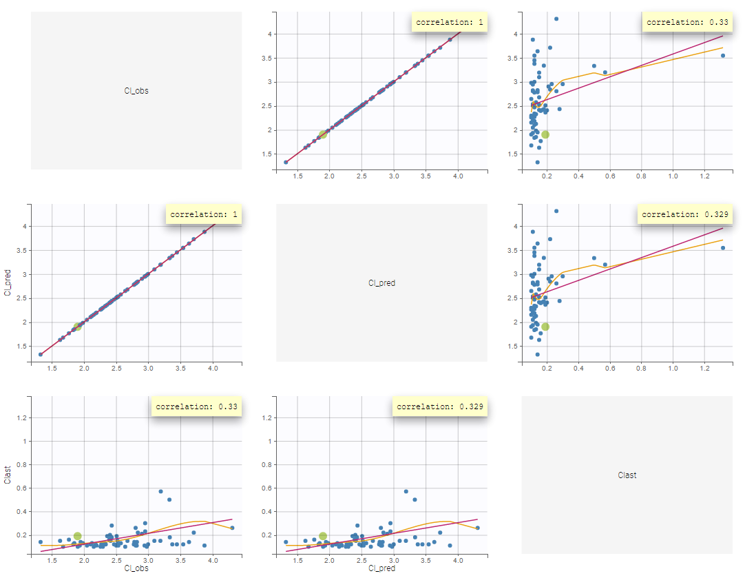
Stratification: coloring and filtering
Stratification can be applied by creating groups of covariate values. As can be seen below, these groups can then be split, colored and/or filtered allowing to check the effect of the covariate on the correlation between two parameters. The correlation coefficient is updated according to the stratifying action. In the following case, We split by the covariate SEX and color bay 2 categories of AGE.

Settings
- General
- Legend and grid : add/remove the legend or the grid. There is only one legend for all plots.
- Information: display/hide the correlation coefficient associated with each scatter plot.
- Display
- Selection. The user can select some of the parameters to display only the corresponding scatter plots. A simple click selects one parameter, whereas multiple clicks while holding the Ctrl key selects a set of parameters.
- Visual cues. Add/remove the regression line or the spline interpolation.
6.2.5.NCA data
Purpose
This plot, available with version 2024, enables the interpreted data for NCA to be displayed in the same way as the observed data. The interpreted data in the plot takes into account exclusions, filters and censoring rules.
While executing the NCA task, the NCA plot is automatically generated alongside the standard set of plots.
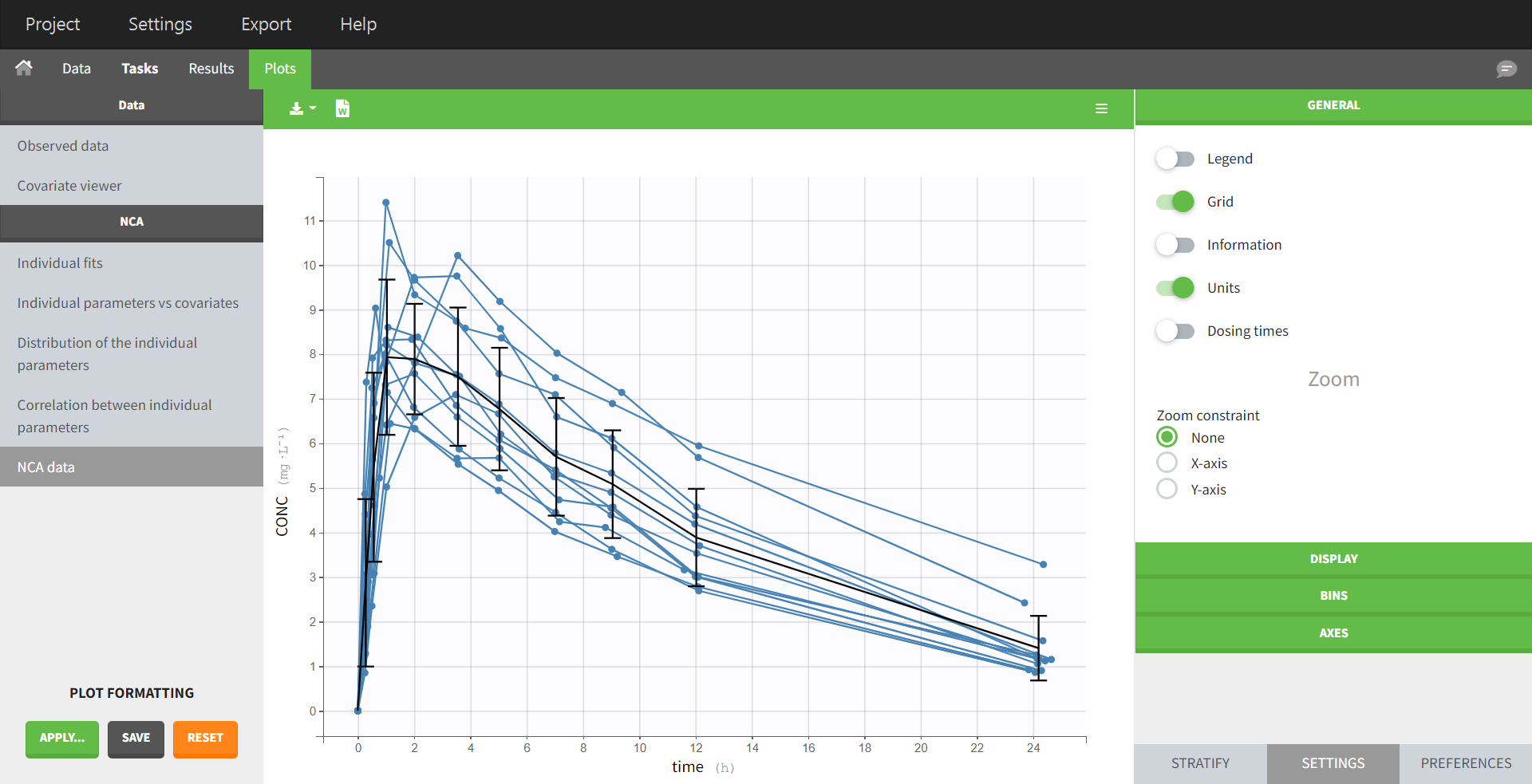 Compared to the Observed data plot, the following data processing rules have been applied:
- additional points at dose time (if not present in original dataset)
- points before the last dose of each profile (i.e occasion or subject) are removed
- BLQ data is replaced according to the chosen NCA settings (BLQ after Tmax and BLQ before Tmax)
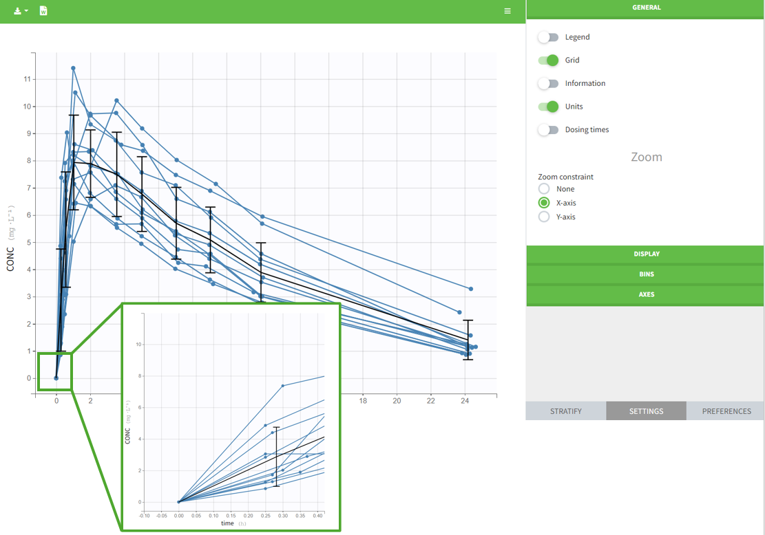 Besides these two mentioned differences from the observed data plot, the NCA data plot offers the same plot settings and stratification properties. Note the option to display the x-axis as nominal time.
Sparse data
The NCA plot for sparse data differs in certain points from the one for dense data.
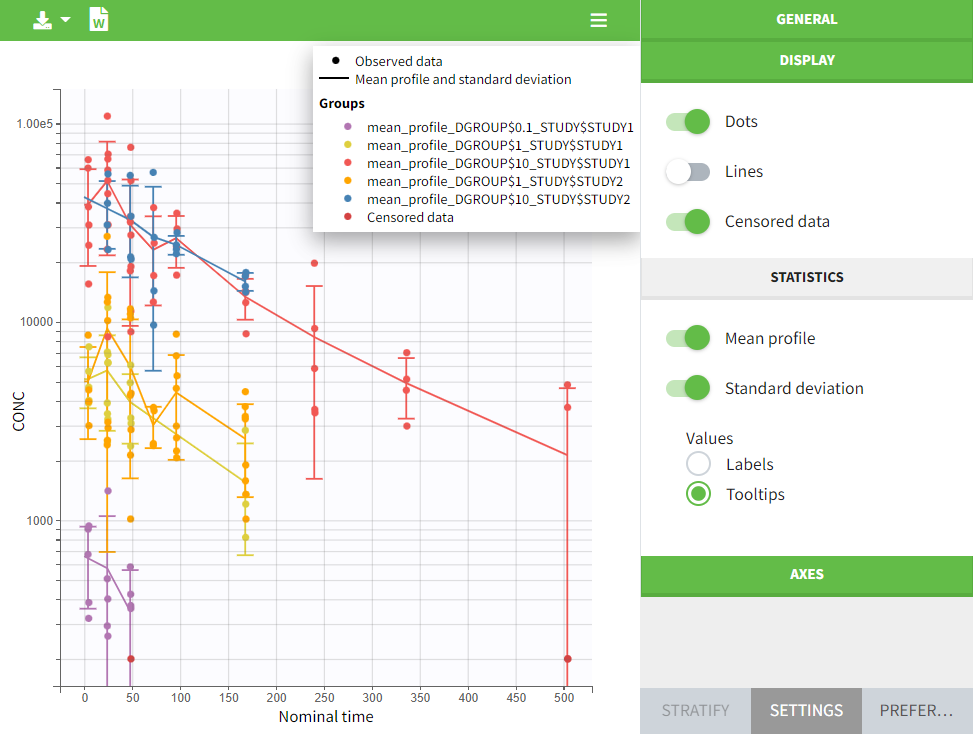
- Stratification
Due to the enforced stratification in the calculation settings, the data also appears according to this stratification in the plots tab. No further stratification settings are possible in the plots tab that deviate from the stratification specified in the calculations panel in the NCA tasks tab.
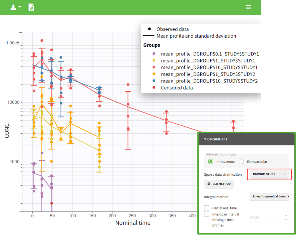
- Trend line
The data is summarized using the arithmetic mean, which is represented by a trend line in the plot. Unlike for dense data in the NCA plot or in the observed data plot, there is no option to select an alternative mean value formula. However, it is possible to display or hide these metrics, arithmetic mean and standard deviation, in the plot using their associated toggles.
- Censored data
The rules defined in the NCA task tab for handling censored data are also considered in the calculation and therefore also in the display of the mean curve and the associated error bars in the in plot.
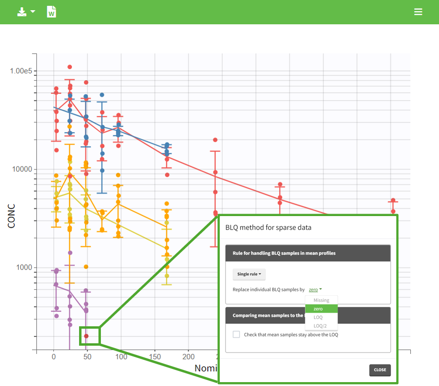
- Nominal time
If nominal time is present in the dataset, it serves as the time variable in calculations and is consequently enforced as the x-axis in the plot, with no option of changing it.
6.3.CA
6.3.1.CA individual fits
Purpose
The figure displays the observed data for each subject, as well as prediction using the individual parameters.
Individual parameters
Information on individual parameters can be used in two ways, as shown below. By clicking on Information (marked in green on the figure) in the General panel, individual parameter values can be displayed on each individual plot. Moreover, the plots can be sorted according to the values for a given parameter, in ascending or descending order (Sorting panel marked in blue). By default, the individual plots are sorted by subject id, with the same order as in the data set.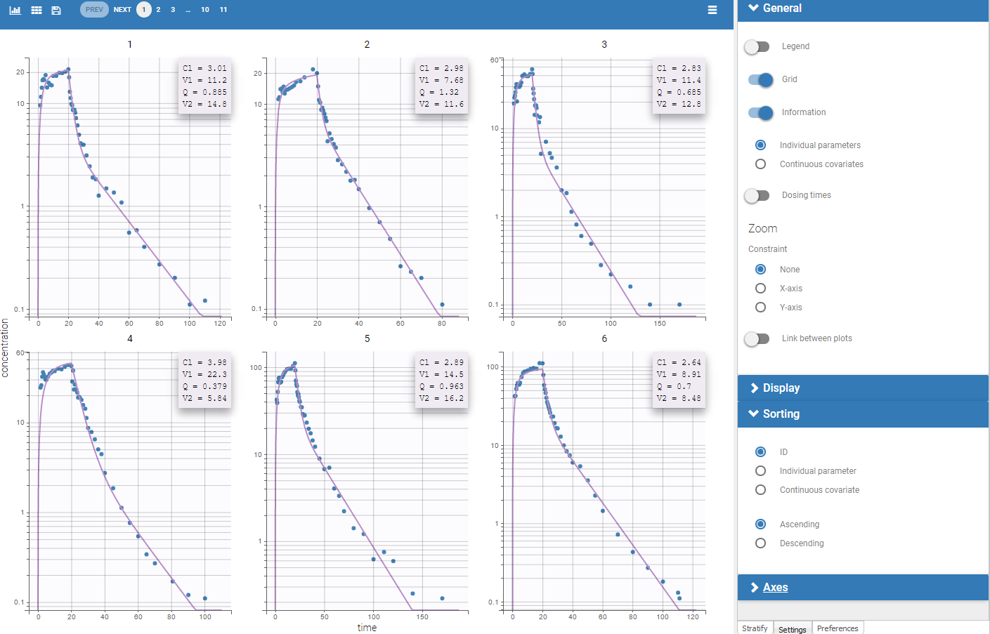
Special zoom
User-defined constraints for the zoom are available. They allow to zoom in according to one axis only instead of both axes. Moreover, a link between plots can be set in order to perform a linked zoom on all individual plots at once. This is shown on the figure below with observations from the remifentanil example, and individual fits from a two-compartment model. It is thus possible to focus on the same time range or observation values for all individuals. In this example it is used to zoom on time on the elimination phase for all individuals, while keeping the Y axis in log scale unchanged for each plot.
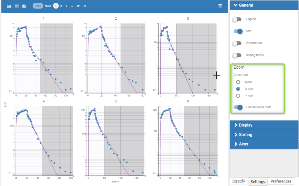
-
Censored data
When a data is censored, this data is different to a “classical” observation and has thus a different representation. We represent it as a bar from the censored value specified in the data set and the associated limit.
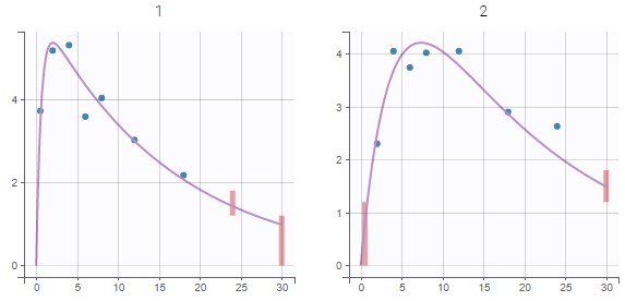
Settings
- Grid arrange. The user can define the number of subjects that are displayed, as well as the number of rows and the number of columns. Moreover, a slider is present to be able to change the subjects under consideration.
- General
- Legend: hide/show the legend. The legends adapts automatically to the elements displayed on the plot. The same legend box applies to all subplots and it is possible to drag and drop the legend at the desired place.
- Grid : hide/show the grid in the background of the plots.
- Information: hide/show the individual parameter values for each subject (conditional mode or conditional mean depending on the “Individual estimates” choice is the setting section “Display”).
- Dosing times: hide/show dosing times as vertical lines for each subject.
- Link between plots: activate the linked zoom for all subplots. The same zooming region can be applied on all individuals only on the x-axis, only on the Y-axis or on both (option “none”).
- Display
- Observed data: hide/show the observed data.
- Censored intervals [if censored data present]: hide/show the data marked as censored (BLQ), shown as a rectangle representing the censoring interval (for instance [0, LOQ]).
- Split occasions [if IOV present]: Split the individual subplots by occasions in case of IOV.
- Number of points of the calculation for the prediction
- Sorting: Sort the subjects by ID or individual parameter values in ascending or descending order.
By default, only the observed data and the individual fits are displayed.
6.3.2.Distribution of the CA parameters
Purpose
This figure can be used to see the empirical distribution of the CA parameters. Further analysis such as stratification by covariate can be performed and will be detailed below.
PDF and CDF
It is possible to display the theoretical distribution and the histogram of the empirical distribution as proposed below.
 The distributions are represented as histograms for the probability density function (PDF). Hovering on the histogram also reveals the density value of each bin as shown on the figure below
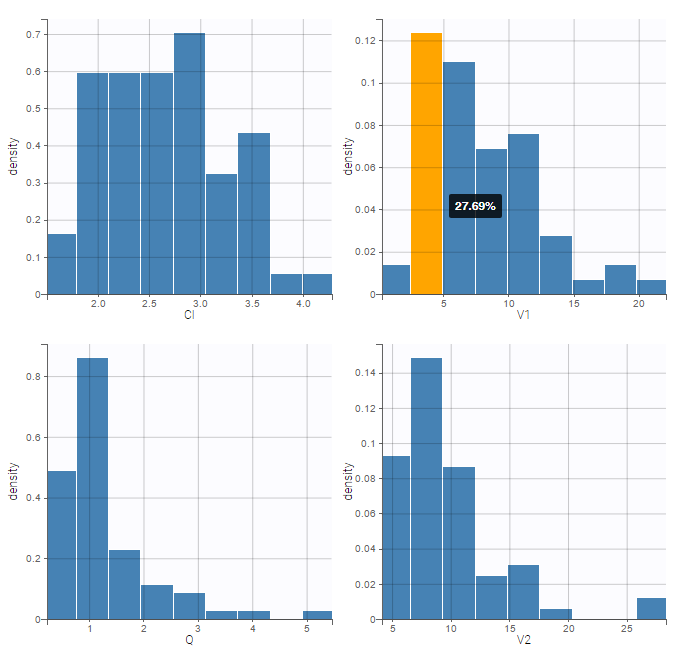
Cumulative distribution functions (CDF) is proposed too.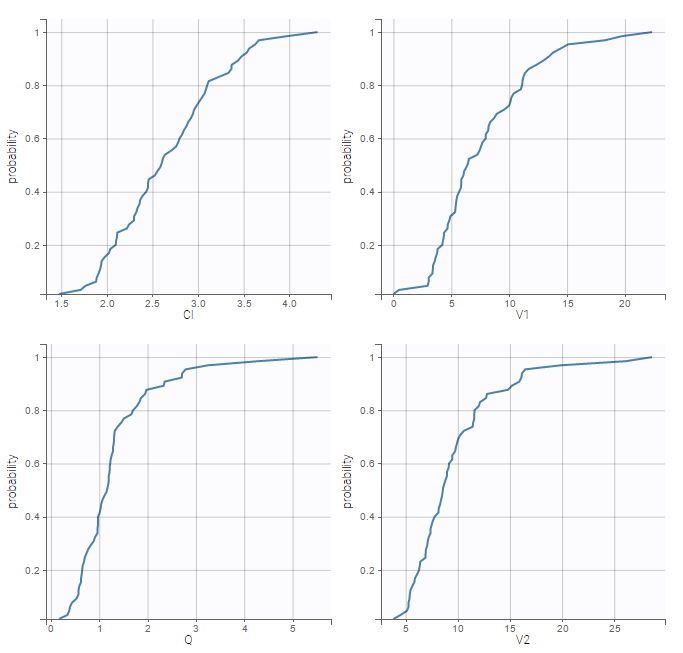
Example of stratification
It is possible to stratify the population by some covariate values and obtain the distributions of the individual parameters in each group. This can be useful to check covariate effect, in particular when the distribution of a parameter exhibits two or more peaks for the whole population. On the following example, the distribution of the parameter k from the same example as above has been split for two groups of individuals according to the value of the SEX, allowing to visualize two clearly different distributions.
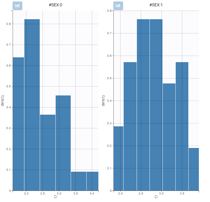 Settings
- General: add/remove the legend, and the grid
- Display
- Distribution function: The user can choose to display either the probability density function (PDF) as histogram or the cumulative distribution function (CDF).
6.3.3.CA parameters vs covariates
Purpose
The figure displays the individual parameters as a function of the covariates. It allows to identify correlation effects between the individual parameters and the covariates.
Identifying correlation effects
In the example below, we can see the parameters Cl and V1 with respect to the covariates: the weight WT, the age AGE and the sex category.
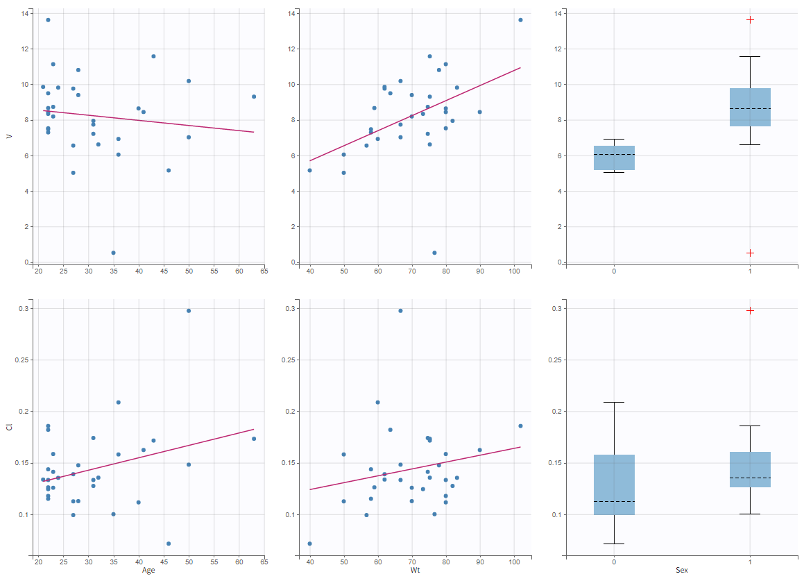
Visual guidelines
In order to help identifying correlations, regression lines, spline interpolations and correlation coefficients can be overlaid on the plots for continuous covariates. Here we can see a strong correlation between the parameter Cl and the age and the weight. This is the same with V1.
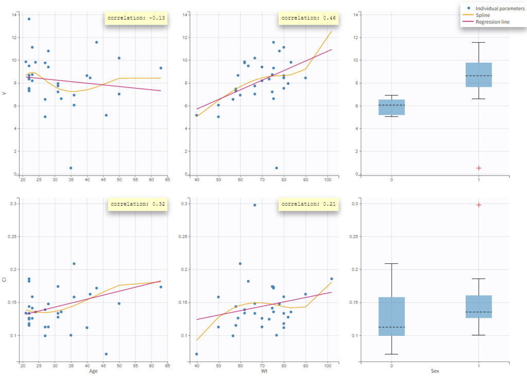
Highlight
Hovering on a point reveals the corresponding individual and, if multiple individual parameters have been simulated from the conditional distribution for each individual, highlights all the points points from the same individual. This is useful to identify possible outliers and subsequently check their behavior in the observed data.
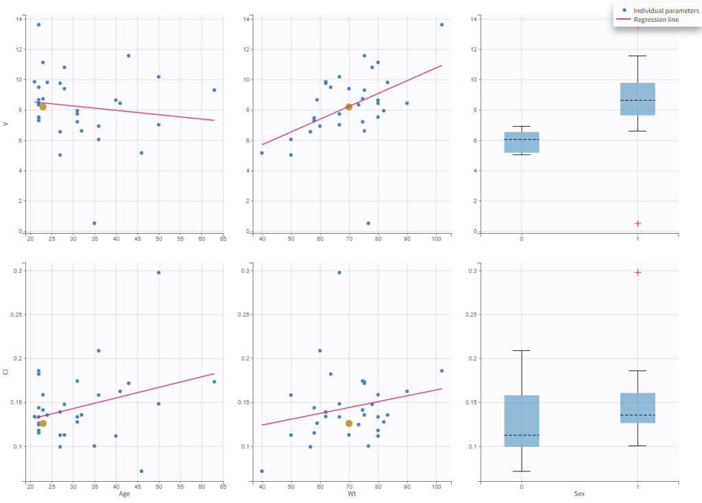
Selection
It is possible to select a subset of covariates or parameters, as shown below. In the selection panel, a set of contiguous rows can be selected with a single extended click, or a set of non-contiguous rows can be selected with several clicks while holding the Ctrl key. This is useful when there are many parameters or covariates.
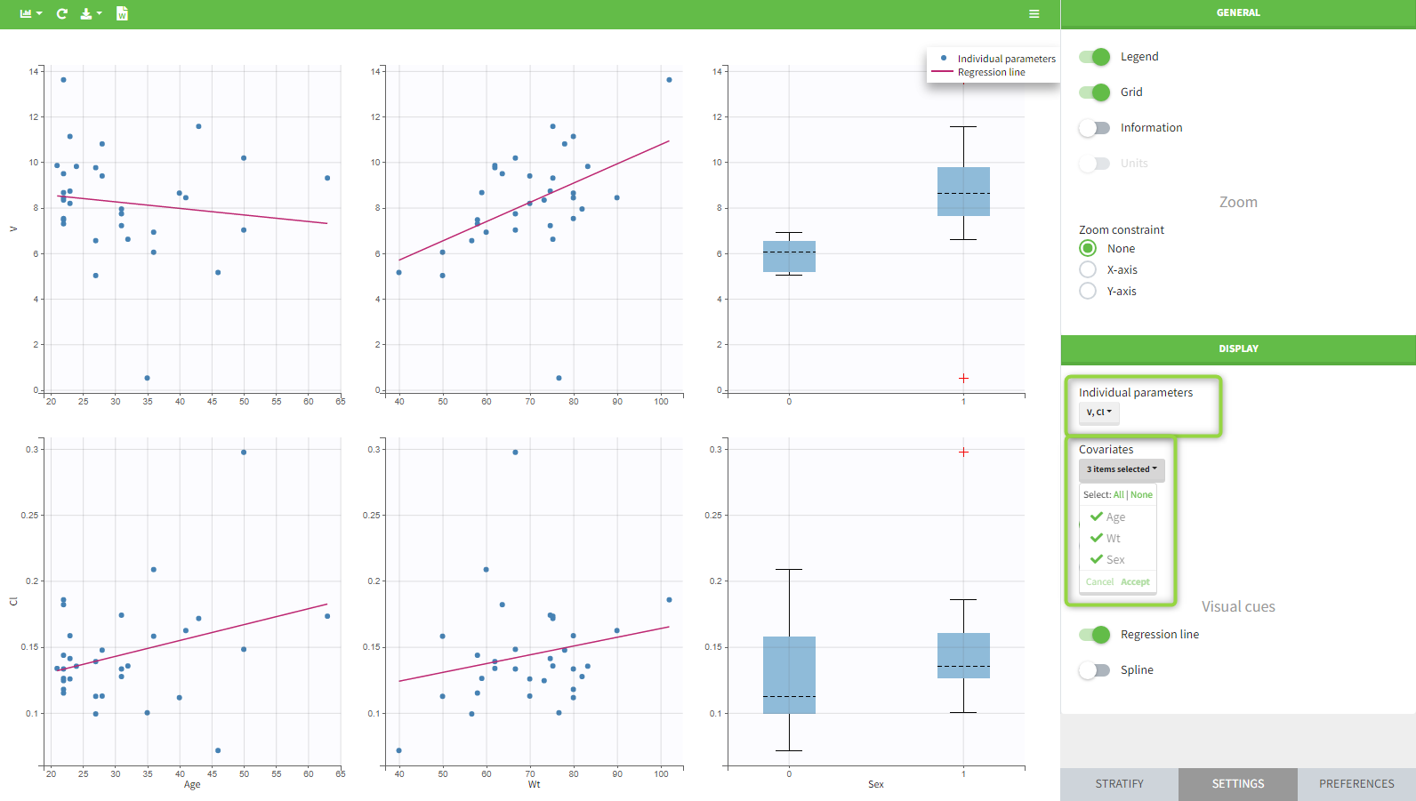
Stratification
Stratification can be applied by creating groups of covariate values. As can be seen below, these groups can then be split, colored or filtered, allowing to check the effect of the covariate on the correlation between two parameters. The correlation coefficient is updated according to the split or filtering.
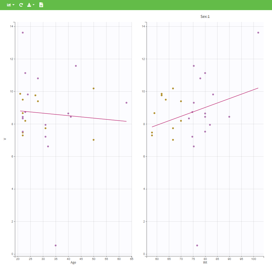
Settings
- General
- Legend and grid : add/remove the legend or the grid. There is only one legend for all plots.
- Information: display/hide the correlation coefficient associated with each scatter plot.
- Display
- Selection. The user can select some of the parameters or covariates to display only the corresponding plots. A simple click selects one parameter (or covariate), whereas multiple clicks while holding the Ctrl key selects a set of parameters.
- Visual cues. Add/remove a regression line or a spline interpolation.
6.3.4.Observations vs predictions plot
The observations vs predictions plot displays observations (\(y_{ij}\)) versus the corresponding predictions (\(\hat{y}_{ij}\)) estimated by the CA task. It is a useful tool to detect misspecifications in the structural model. The points shall scatter as close as possible along the y = x line (black solid line). If a large amount of points are not scattered close to the identity line, then this might be due to the chosen structural model not capturing certain kinetics. Moreover, the distribution of the dots should be symmetrical around the y=x line, meaning that the model prediction is sometimes abve and sometimes below the observed data.
This plot is generated automatically when you run the compartmental analysis task. You can access it from the CA section in the plots list.
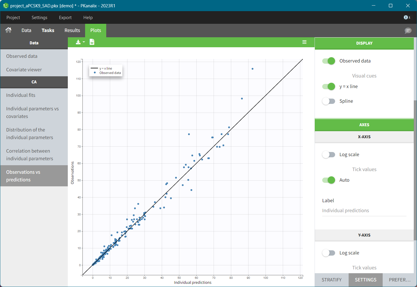
Visual Guides
In addition to the observed data, in the DISPLAY settings panel you can add: the identity line y = x and spline interpolation.
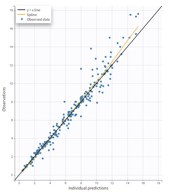
Highlight
Hovering on any point of observed data shows:
- the subject id and time corresponding to this point
- highlights all the points corresponding to this subject
- segments linking all points corresponding to the same individual to visualize the time chronology.
Highlighting works across plots. An individual data highlighted in this plot, will be highlighted in every other plot to help you in the model diagnosis.
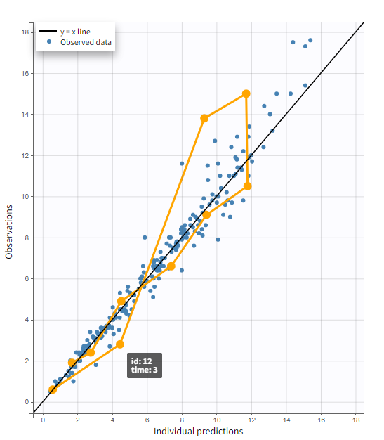
Log scale
A log scale allows to focus on low observation values. You can set it in the AXIS section of the settings panel for each axis separately or for both together.
The example below displays the predicted concentrations of remifentanil, modeled via a two-compartments model with a linear elimination. In this case, the log-log scale reveals a misspecification of the model: the small observations are under-predicted. These observations correspond to late time points, meaning that the last phase of elimination is not properly captured by the two-compartment model. A three-compartment model might give better results.
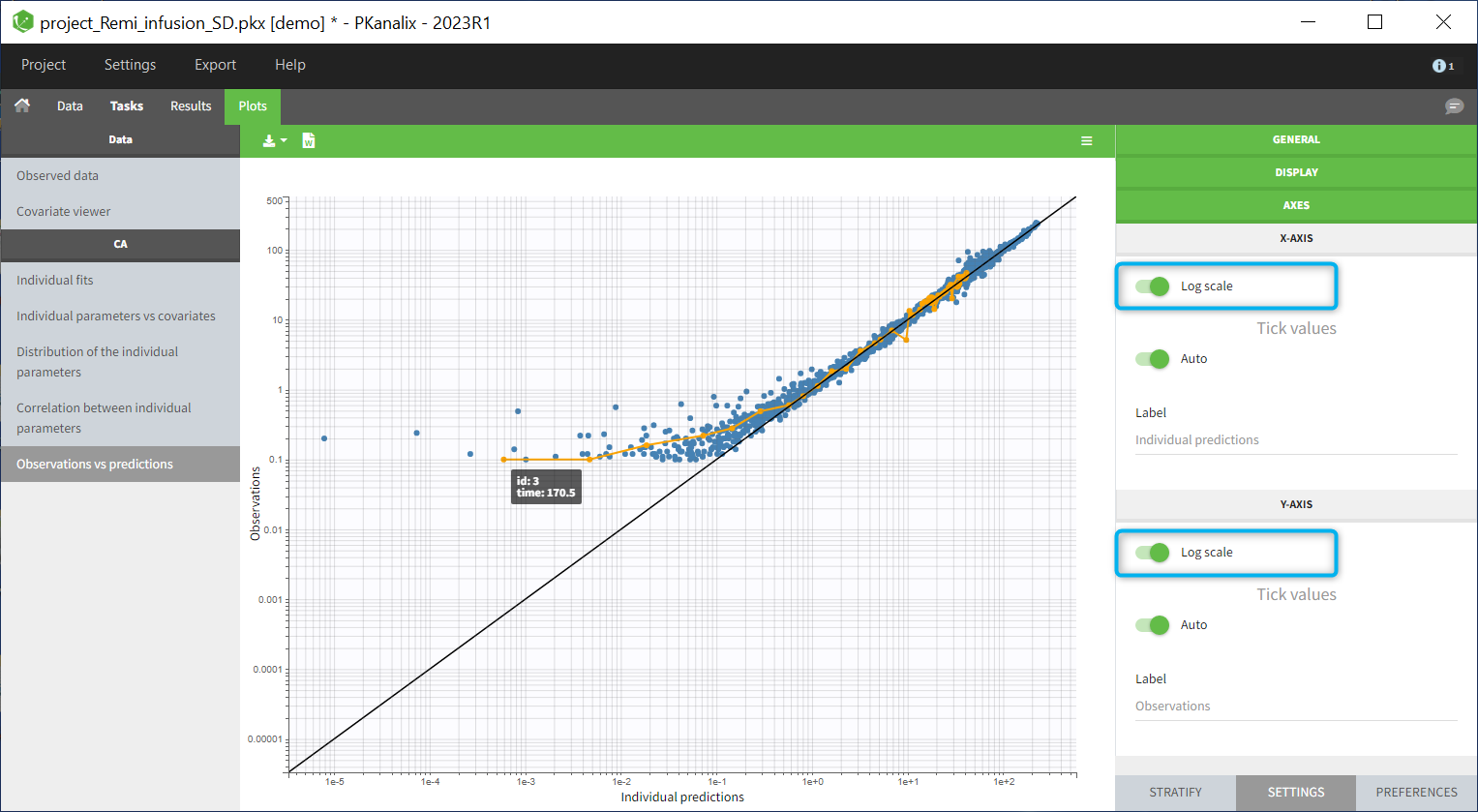
Settings
- General
- Legend and grid : add/remove the legend or the grid.
- Display
- BLQ data : show and put in a different color the data that are BLQ (Below the Limit of Quantification)
- Visual cues: add/remove visual guidelines such as the line y = x or a spline interpolation.
- Axis
- Use log scale
- Set automatic or manual (user – defined step) tick values
- Edit axis labels
Stratification
You can split, color or filter the plot as described for the observed data.
6.3.5.Correlation between CA parameters
Purpose
This plot displays scatter plots for each pair of parameters. It allows to identify correlations between parameters, which can be used to see the results of your analysis and see the coherence of the parameters for each individuals.
Example
In the following example, one can see pairs of parameters estimated for all parameters.
 Visual guidelines
In addition to regression lines, correlation coefficients can been added to see the correlation between random effects, as well as spline interpolations.
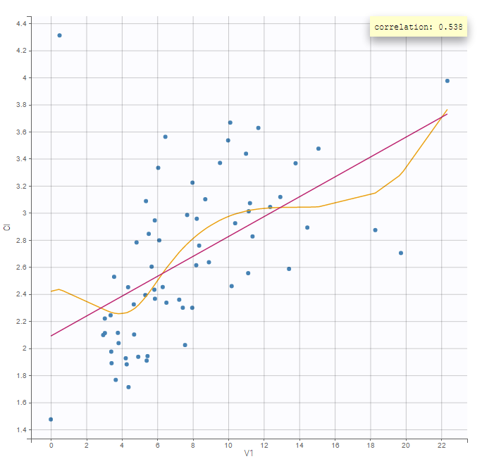
Selection
It is possible to select a subset of parameters, whose pairs of correlations are then displayed, as shown below. In the selection panel, a set of contiguous rows can be selected with a single extended click, or a set of non-contiguous rows can be selected with several clicks while holding the Ctrl key.
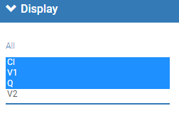
Highlight
Similarly to other plots, hovering on a point provides information on the corresponding subject id, and highlights other points corresponding to the same individual.
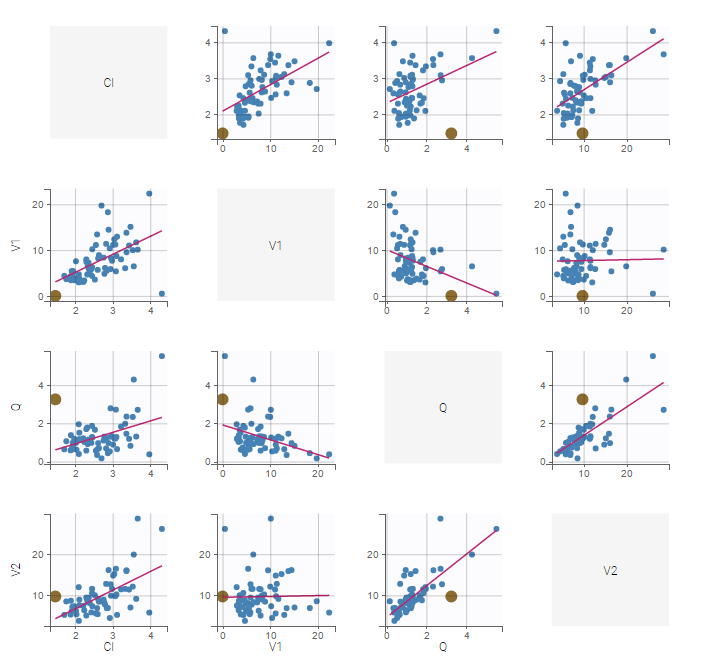
Stratification: coloring and filtering
Stratification can be applied by creating groups of covariate values. As can be seen below, these groups can then be split, colored and/or filtered allowing to check the effect of the covariate on the correlation between two parameters. The correlation coefficient is updated according to the stratifying action. In the following case, We split by the covariate SEX and color bay 2 categories of AGE.
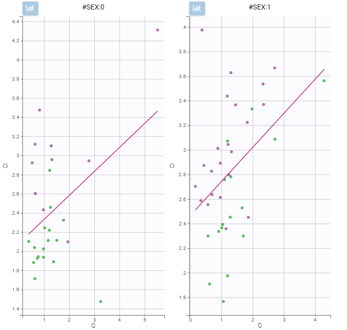
Settings
- General
- Legend and grid : add/remove the legend or the grid. There is only one legend for all plots.
- Information: display/hide the correlation coefficient associated with each scatter plot.
- Display
- Selection. The user can select some of the parameters to display only the corresponding scatter plots. A simple click selects one parameter, whereas multiple clicks while holding the Ctrl key selects a set of parameters.
- Visual cues. Add/remove the regression line or the spline interpolation.
6.4.Bioequivalence
6.4.1.Sequence-by-period plot
Purpose
The sequence-by-period plot allows to visualize, for each parameter, the mean and standard deviation for each period, sequence and formulation.
Description
For each formulation, period and sequence (as defined in the Bioequivalence settings), the mean and standard deviation is displayed. The dots are colored according to the formulation, and dots belonging to the same sequence connected by lines. Dots are placed on the x-axis according to the occasion value.
If the parameter has a log-transform (see Bioequivalence settings), the dots represents the geometric mean and the error bars */ the geometric standard deviation. If the parameter is not log-transformed, the dots represent the arithmetic mean and the error bars +/- the standard deviation. NCA parameter values being NaN are excluded and a warning message is displayed.
The example below shows a repeated crossover with sequences RTRT and TRTR. Three NCA parameters are displayed.
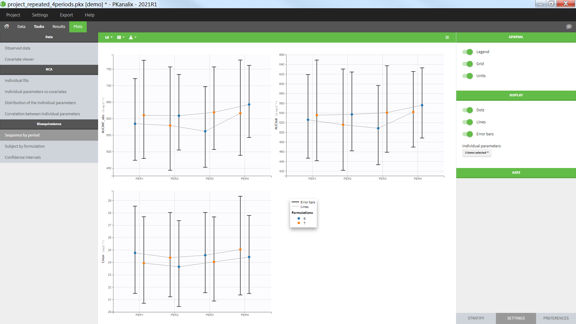
Troubleshooting
- The connecting lines to do appear:
If the plot setting “Lines” in selected and the connecting lines do not appear, it is because no categorical covariate column as been defined as “Sequence” in the Bioequivalence settings.
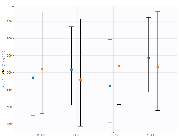
- There are vertical connecting lines:
This means that the column defined as “Sequence” in the Bioequivalence settings is not consistent with the sequence of formulation according to the Occasion column. In the tab “Data”, you can define an “additional covariate” and select the “covariate sequence (XXX)” with XXX being the column representing the formulation. Then use this column as “Sequence” when defining the factors in the model.
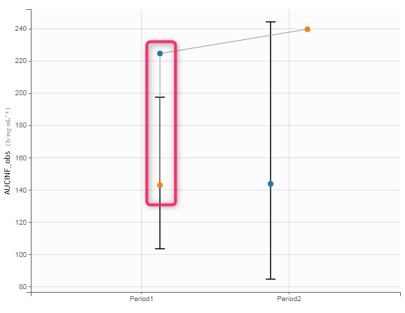
- There are several periods on the x-axis although no column was indicated as “period” in the Bioequivalence settings:
When no column is indicated as “period”, we use the column tagged as “occasion” in the data set. If no column has been tagged as “occasion” (parallel design), the occasion is considered to be 1 for all individuals.
Settings
- General
- Legend: hide/show the legend. The legends adapts automatically to the elements displayed on the plot. The same legend box applies to all subplots and it is possible to drag and drop the legend at the desired place.
- Grid : hide/show the grid in the background of the plots.
- Units: hide/show the units of the NCA parameters. Note that the color and surrounding character can be chosen in the plot “Preferences”.
- Display
- Dots: hide/show the dots representing the means
- Lines: hide/show the lines connecting the dots belonging to the same sequence
- Error bars: hide/show the error bars representing the standard deviation
- Individual parameters: select which individual parameters to show on the plot
Stratify
This plot can be split and filtered by the covariates but not colored. The categorical covariate indicated of Formulation in the Bioequivalence settings is automatically used to color the dots. The colors can be changed in the plot “Preferences > Formulations”:
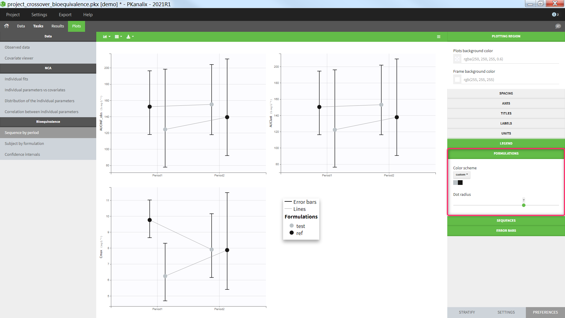
6.4.2.Subject-by-formulation plot
Purpose
This plot allows to visualize, for each parameter, the subject-by-formulation interaction and the inter-subject variability.
Description
Each subplot corresponds to one NCA parameter and one non-reference (test) formulation. The individual parameter values for the test and reference formulations are displayed side by side. Values corresponding to the same individual are connected by a line. When an individual has received several times the same formulation (repeated crossover), the average for each formulation is calculated and plotted.

Settings
- General
- Legend: hide/show the legend. The legends adapts automatically to the elements displayed on the plot. The same legend box applies to all subplots and it is possible to drag and drop the legend at the desired place.
- Grid : hide/show the grid in the background of the plots.
- Units: hide/show the units of the NCA parameters. Note that the color and surrounding character can be chosen in the plot “Preferences”.
- Display
- Dots: hide/show the dots representing the individual parameter values
- Lines: hide/show the lines connecting the dots belonging to the same individual
- Individual parameters: select which individual parameters to show on the plot
Stratify
The plot can split and filtered but not (yet) colored.
6.4.3.Confidence intervals plot
Purpose
This plot allows to visualize the confidence interval for the ratio for each parameter, as well as the BE limits. Confidence intervals within the BE limits are shown in green while the others are shown in red.
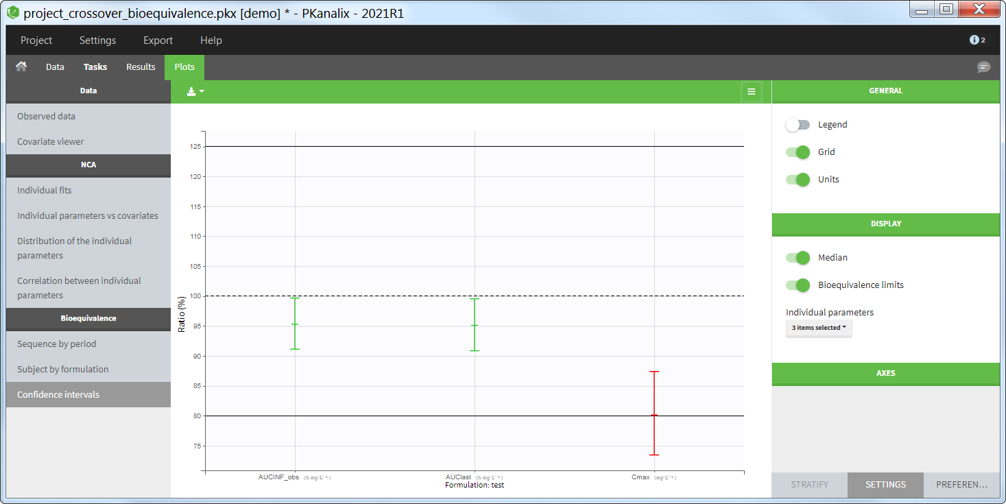
Settings
- General
- Legend: hide/show the legend. The legends adapts automatically to the elements displayed on the plot. The same legend box applies to all subplots and it is possible to drag and drop the legend at the desired place.
- Grid : hide/show the grid in the background of the plots.
- Units: hide/show the units of the NCA parameters. Note that the color and surrounding character can be chosen in the plot “Preferences”.
- Display
- Median: hide/show the line at ratio=100%.
- Bioequivalence limits: hide/show the horizontal lines at the BE limits, which can be set in the BE settings
- Individual parameters: select which individual parameters to show on the plot
Stratify
This plot cannot be stratified by covariates.
6.5.Transferring plot formatting within one project or across projects
Note: the features described on this page are not available in MonolixSuite versions prior to 2024R1.
MonolixSuite offers the ability to transfer plot formatting from one plot to another within the same project or across projects. This can save you time and effort when you want to apply the same formatting options, such as stratification, preferences, or settings, to multiple plots, or when you want to use the same plot formatting for different analyses or datasets.
- Transferring plot formatting within one project
- Transferring plot formatting across projects with plot presets
- Applying pre-defined plot formatting
- Restoring default plot formatting
Transferring plot formatting within one project
To transfer plot formatting within one project, you need to use the “Apply…” button on the bottom left of the Plots tab and select “From plot” in the window that opens:
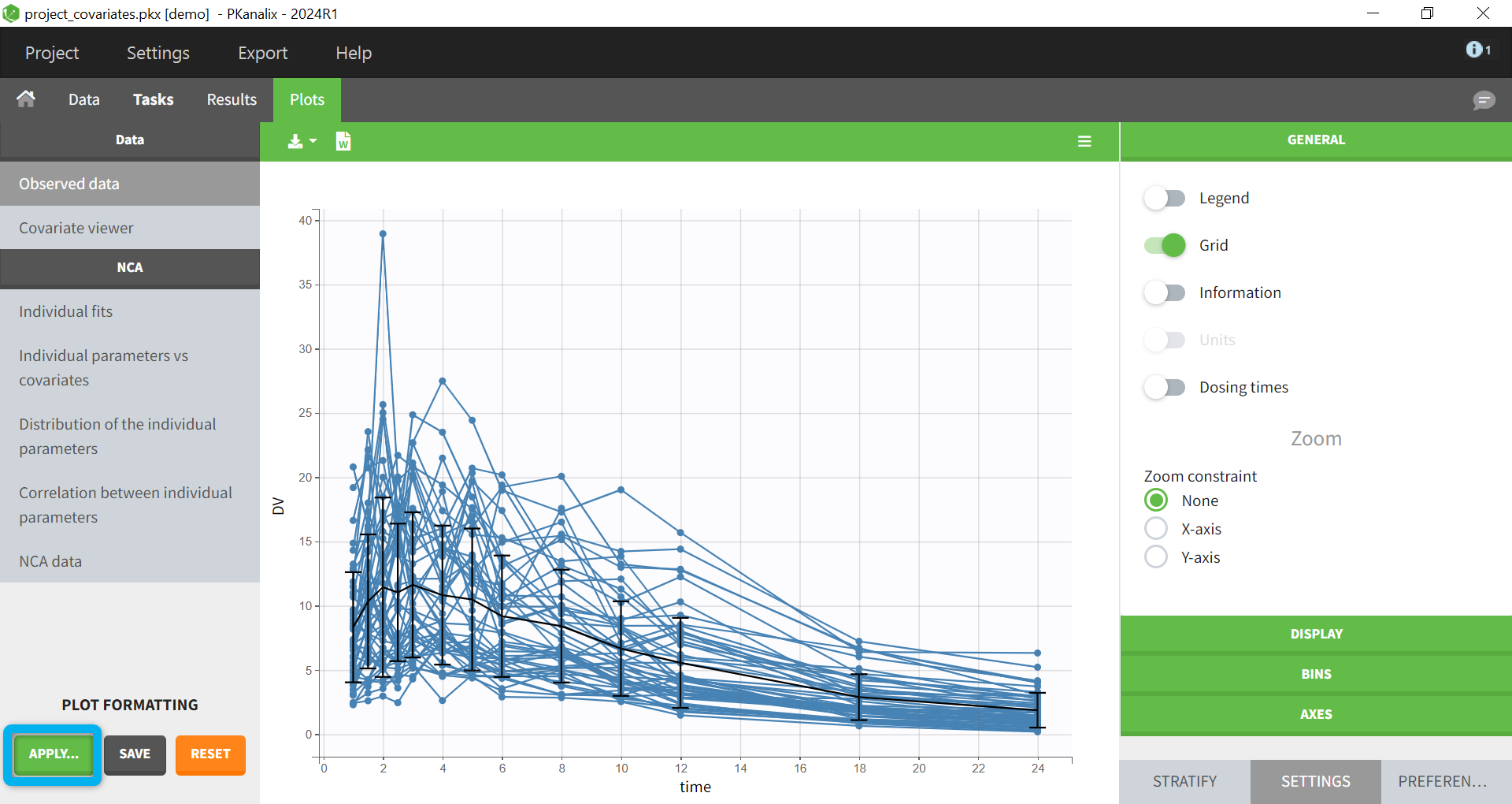
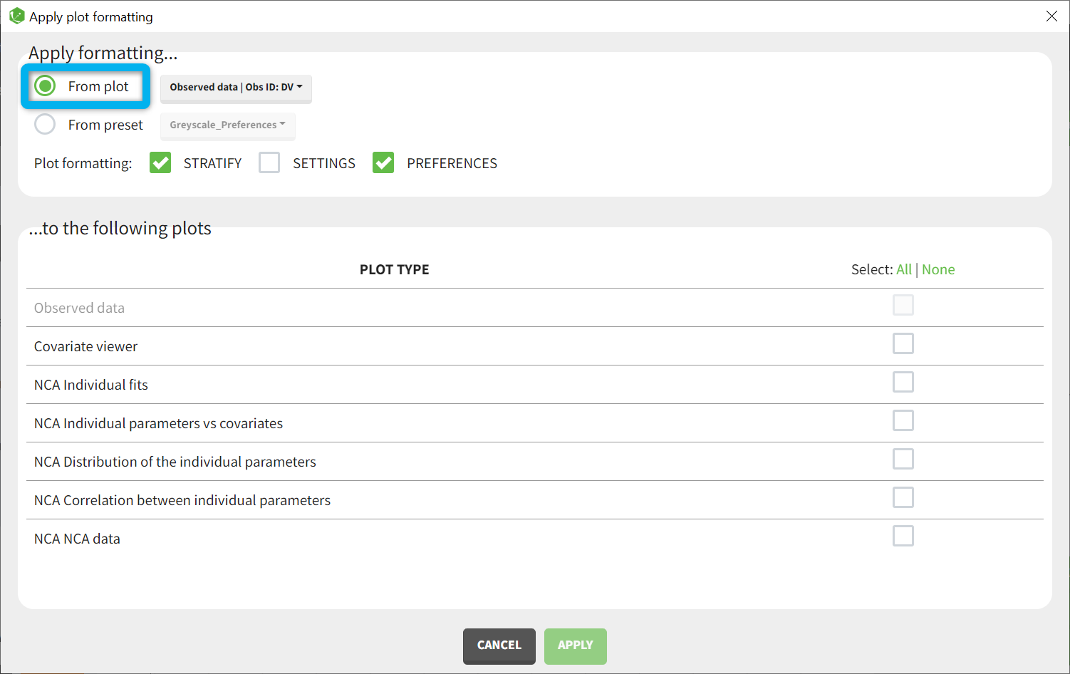
Selecting the source and target plots
The window allows you to select the source plot, which is the plot that has the formatting you want to transfer, and the target plots, which are the plots that you want to apply the formatting to. You can select all plots by clicking on the Select all button, or select all plots specific to some observation id with the “Fast selection”.

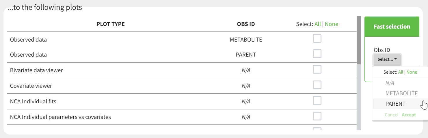
Choosing the sections to transfer
You can also choose which sections of the configuration you want to transfer: Stratify, Settings, or Preferences.
![]()
By default, Stratify and Preferences are selected.
- The Stratify section includes the options to stratify the plots by covariates or occasions.
- The Settings section includes the options to customize the content of the plots: elements displayed or not on the plots, such as the legend, the grid, the observed data points, etc, and calculation settings such as the axes, bins etc.
- The Preferences section includes the options to change the colors, fonts, sizes, etc.
Once you have selected the source plot, the target plots, and the sections to transfer, you can click on the Apply button to transfer the plot configurations.
Transferring plot formatting across projects with plot presets
To transfer plot formatting across different projects, you need to use the plot presets feature, which allows you to define and apply presets for plot configurations.
Defining a plot preset
To define a plot preset, you need to first set up your plot configuration as you would like by choosing the stratification, preferences, and settings options for each plot (you can use the transfer or plot formatting between plots within the same project, described in the first section, to help you). Then, you can save this configuration as a preset by clicking on the Save icon in the Apply from the Plot Formatting panel:

You will be asked to give a name and a description to your preset, and to select which sections of the formatting you want to include in the preset among Stratify, Settings and Preferences. If the project has several types of observations, only the plots corresponding to one of them can be used to define the preset so it is necessary to select the observation id. You can also choose to set this preset as your default, which means that when you click on Reset, the plot formatting from this preset will be applied instead of the system default.
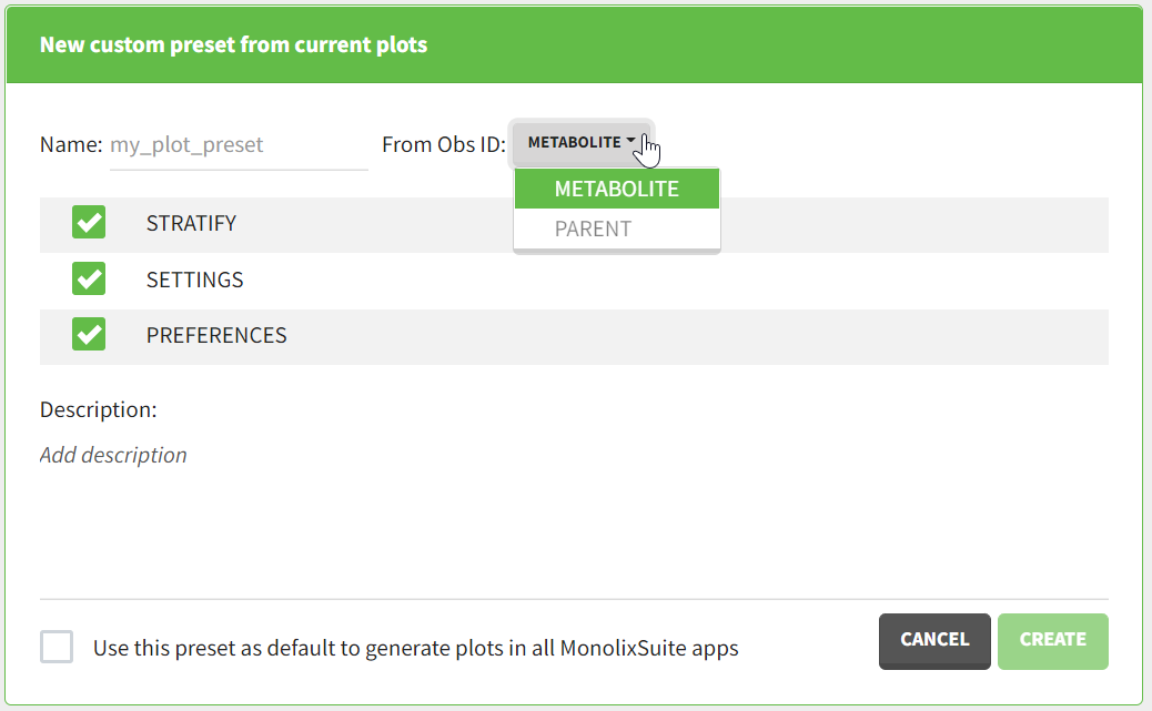
Applying a plot preset
After saving your preset, it will be available in the list of presets that you can choose from when you click on “From preset” in the window that opens with “Apply…” in the Plot Formatting panel.
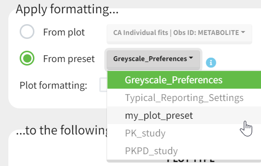
You can apply your preset to a list of plots in another project, by opening this project, clicking on “Apply…” and “From preset” and by selecting the preset and the target plots, and finally clicking on Apply. This will transfer the plot configurations from the preset to the target plots.
The target plots must be the same type of plots that were used to define the preset: for example if no CA plot had been generated in the project used to define the preset, then the plot preset cannot be applied to a CA plot in a new project, as there is no CA formatting option to apply.
Note that axis limits values and bins settings are not saved as part of the preset because they are considered too project-specific.
Note this major difference between “Apply formatting from plot” and “Apply formatting from preset”:
- “Apply formatting from plot” applies all selected options from the source plot to all selected target plots. Thus, if you select the NCA data plot stratified by STUDY as source plot and the Observed data plot as target plot, and “Stratify” section in plot formatting to be transfer, you will obtain the Observed data plot stratified by STUDY.
- “Apply formatting from preset” applies the selected options from each plot saved in the preset to the corresponding plot in your project. Thus, if you saved a preset including the “Stratify” section based on a project where the NCA data plot is stratified by STUDY but not the Observed data plot, applying that preset to another project will stratify the NCA data plot by STUDY but not the Observed data plot.
Managing plot presets
You can also manage your presets by going to Settings > Manage presets > Plot formatting.

This will open a window where you can see all presets, modify, update or remove your custom presets, and export or import them as separate files with a lixpst extension. That way you can easily share your presets with your colleagues or collaborators to standardize your plot formatting.

Applying pre-defined plot formatting
In addition to your custom presets, MonolixSuite also provides two pre-defined presets that you can use to apply plot formatting. These presets are:
- Greyscale_Preferences: This preset affects only the Preferences section of the plot configurations, and produces publication-ready greyscale plots with optimized size and spacing of the texts to improve readability of the plots (example shown below for the NCA Individual fits).
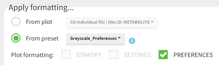

- Typical_Reporting_Settings: This preset affects only the Settings section of the plot configuration, and corresponds to plot settings typically chosen to report the analysis results. It has additional settings for Monolix plots, but in PKanalix it only removes the grid in the background for all plots:

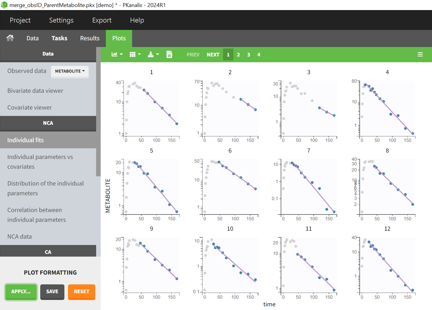
You can apply these presets to any plot in your project by selecting them from the list of presets and clicking on Apply. You can also combine these presets with your own presets or with the Apply from plot feature, to create the plot configuration that suits your needs.
Restoring default plot configuration
Using the Reset button
If you want to restore the default plot configuration, you can click on the Reset icon in the Apply from plot panel. This will reset all plots to the system default, or to your custom default if you have defined one.

Note that resetting the plot configuration will not affect the plot presets that you have defined or imported. You can still apply them to any plot after resetting.
Defining a custom default
To define a custom default, you need to create a preset and select the option “Use this preset as default” when saving it. This will make this preset the default configuration for all plots. You can also unset a preset as default by going to Settings > Manage presets > Plot formatting, and unchecking the option “Use this preset as default” for the preset.
7.Reporting
Starting from the 2023R1 version of the MonolixSuite, PKanalix includes a feature of automated report generation. This feature is available in PKanalix through Export > Generate report. After defining settings in the window that pops up and clicking on the Generate report button, a report in the form of a Microsoft Word (docx) document will be generated in the specified directory. Note that reports generated using command line and lixoftConnectors will contain tables but no plots. Reporting module is not available on CentOS 7.
Here we explain:
- Different strategies for report generation
- How to generate a default report
- How to generate a report using a user-provided template file
- How to rename words and phrases used by PKanalix in generated reports
- How to generate a report using command line arguments
To see examples of a full workflow of report generation in PKanalix, you can visit this page.
Report generation strategies
When selecting Export > Generate report…, there are two different strategies available for report generation:
- Using a default template file – choosing this option will generate the report containing tables of NCA settings, individual NCA metrics, summary of NCA metrics, BE settings and results, CA settings, individual CA parameters, summary of CA parameters and CA cost, as well as all plots available in the interface using their current settings. This option allow to obtain a basic report with all results in one click.
- Using a custom template file – if users choose this option, they will be required to provide a path to the template word file which contains placeholders that will be replaced by tables, plots and keywords when generating the report.
Several other options are available in the pop-up window after the Generate report option is clicked on:
- Document watermark – users can specify a custom text that will appear as a watermark in the report. Font family, font size, color, layout and transparency can be specified, if text is entered into the Text input widget.
- Generated report file – users can choose if the generated report will be saved next to the project file (in that case only the name of the generated report file needs to be given to PKanalix) or in a custom directory (absolute path that includes the generated report file name needs to be given).
- Table styles (only when the custom template file option is selected) – users can choose a style for tables from the list of styles available by default in Microsoft Word. This setting can be overridden by specifying the style directly in the table placeholder. This way custom user-created or company-specific styles can be used.
Default template file
Selecting the option to use the default template file to generate a report gives users a possibility to quickly generate a document containing results of an analysis.
Such a report will consist of:
- name of the PKnaalix project
- data set file name,
- a date of report generation,
- a table containing settings used in NCA analysis (if NCA was run),
- a table of individual NCA parameters with mean and CV% (if NCA was run),
- a table with a summary of NCA parameters (if NCA was run),
- a table with BE settings (if BE was run),
- a table with results of BE analysis (if BE was run),
- a table of compartmental analysis (CA) calculation settings (if CA was run),
- a table of individual CA parameters and costs with mean and CV% (if CA was run),
- a table with a summary of CA parameters (if CA was run),
- a table with total cost, -2LL, AIC and BIC (if CA was run),
- all plots displayed in the GUI with settings currently defined in the interface.
By clicking on View default template, a Word document containing placeholders for all the elements that will be present in the generated report can be downloaded. This document can then be used as a basis for the creation of a custom template file.
Custom template file
The option to use the custom template file can be selected if a user has previously created a Word document (a template) that typically contains placeholders to be replaced by project-specific information, such as tables of results, plots or settings used in a project. Placeholders are strings with a specific syntax that define the settings and layout with which tables and plots will be generated during the report generation process.
For example, in the picture below, a template file on the right contains a placeholder for the observed data plot. So, after report generation, the report file on the right contains a plot for the observed data instead of this placeholder.

Using placeholders
There are three types of placeholders that can be used:
Placeholders for project settings are of format %keyword% and, during the report generation step, they will be replaced by project or global PKanalix settings. For example, if a custom template file contains the placeholder %NCA_integralMethod%, this placeholder will be replaced by the integral method (e.g “linear up log down”) used by a PKanalix project for which the report is being generated. The list of all project settings placeholders can be found here.
Placeholders for plots are of format <lixoftPLH>settings</lixoftPLH> and, during the report generation step, they will be replaced by plots that are available in the PKanalix user interface. Placeholders for plots contain settings that describe how the generated plots should look like. All settings that are available for plots in the interface are available in reporting as well, with addition of several others that describe plot dimensions and display of captions. The list of the main plot settings placeholders can be found here.
Placeholders for tables are also of format <lixoftPLH>settings</lixoftPLH>. Placeholders for tables contain settings that describe how the generated table should look like and they allow more flexibility in the layout compared to the display of tables in the GUI. Indeed, table placeholders can contain settings that result in generated tables being different from the ones available in the Results tab of the PKanalix interface, such as an option to choose which rows or columns to include in the table, or to split tables in a different direction that the one present in interface. Here is the list of all settings that can be used for table placeholders.
Placeholders do not need to be written by the users. They can be generated through the interface, using the Copy reporting placeholder (![]() ) button which can be found next to every plot and results table. Clicking on this button will display the corresponding placeholder in a pop-up window. The displayed placeholder can then be copied to a template file and will be replaced by the table or plot, exactly as they are shown in the interface, with all stratification options and display settings applied.
) button which can be found next to every plot and results table. Clicking on this button will display the corresponding placeholder in a pop-up window. The displayed placeholder can then be copied to a template file and will be replaced by the table or plot, exactly as they are shown in the interface, with all stratification options and display settings applied.
Let’s take a look at how “Copy reporting placeholder” buttons work on a specific example. If we load the demo project_censoring.pkx, go to the Observed data plot and click on the Copy reporting placeholder button above the plot, a pop-up window will appear containing the placeholder for the plot, which can then be used in a report template to generate the plot that looks exactly like the plot currently shown in the interface. As you can see on the screenshot below, the placeholder contains information about plot type, plot size, caption and axes labels.


If we now close the pop-up, enable legend and open the pop-up again, the placeholder will contain the enabled legend setting and, if we put the placeholder in a report template, the generated plot will have a legend present in its corner, as shown in the screenshot on the right.


If we would like our report to have the Observed data plot stratified by a categorical covariate, STUDY, we can stratify the plot in the interface and click on the Copy reporting placeholder button again to generate a placeholder for this plot, as shown on the images below. You can notice that the generated placeholder now contains settings stratification and layout, which control stratification and plot layout.


There are several options present inside the “Placeholder for Report Template” pop-up:
- indent – determines number of spaces used for indentation of settings in the placeholder,
- flow level – determines the compactness of placeholders, i.e how often we start a new line (lower the number, more compact the placeholder will be),
- dimensions units – gives the ability to choose if width and height will be in cm or inches,
- lock aspect ratio – if on, changing width or height will change the other dimension to keep the aspect ratio present on the screen.
It is possible to edit placeholders directly inside the pop-up. Clicking on the Preview button will generate and open a Word document containing a plot or a table described with the placeholder. This option is especially useful when a user manually modifies placeholders, to check if the syntax and the behavior are correct.
Copy to clipboard button will copy the placeholder with the <lixoftPLH> tag, ready to be pasted to the custom Word template.
Using areTaskResultsAvailable
Besides placeholders, templates can include the areTaskResultsAvailable tag, which can be used to display part of the template conditionally in the report.
For example, if a template contains the text:
<? areTaskResultsAvailable(nca) ?>
Show this if NCA has been run
</?>
The text “Show this if NCA has been run” will be present in the generated report, only if NCA results are available, otherwise the tags and the text will not be present in the generated report. Besides text, it is possible to include placeholders inside the areTaskResultsAvailable tag. Keywords that can be used inside the parentheses are “nca” for non-compartmental analysis, “be” for bioequivalence and “ca” for compartmental analysis.
Renamings
In the PKanalix Preferences, there is an option to replace default names of NCA parameters by custom names (see screenshot below). Changing these options will change the names in the interface (after restarting the program) and in generated reports.
A section Reporting placeholder entry renamings in Preferences can be used to change words and phrases that will appear in generated reports by default. For example, if we give alias “LeastSquareMean” to a placeholder entry “AdjustedMean”, the word “AdjustedMean” in the BE table generated by the reporting feature will be replaced by the word “LeastSquareMean”.
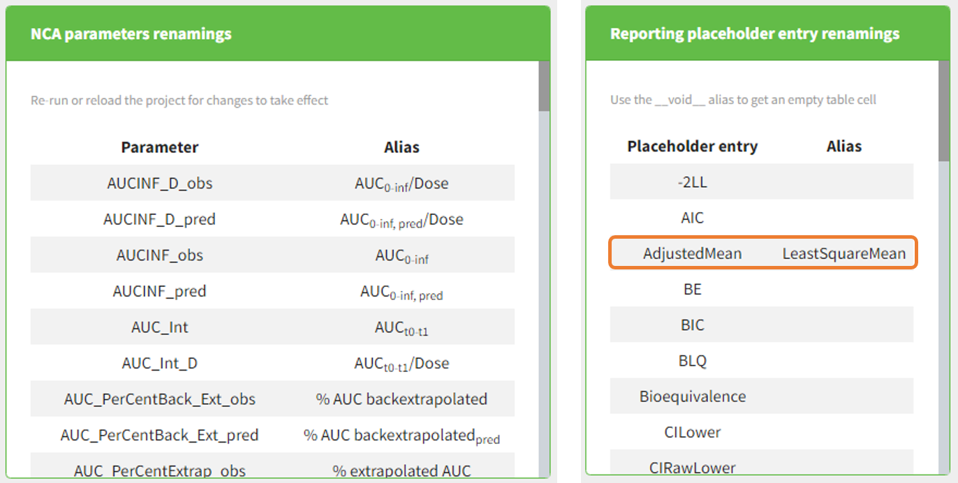
In addition, it is possible to rename words found in generated tables, by specifying an argument renamings inside the placeholder. This allows users to change words present in the data set as well. For example, if an imported data set contains a column “Formulation” with values T (for the test drug) and R (for the reference drug), specifying the following inside a placeholder will replace all occurrences of word “T” inside the table with “test” and “R” with “reference”:
renamings:
    T: test
    R: reference
For categorical covariates, it is possible to specify both the covariate name and the covariate modality to be repaced, in order to avoid ambiguities if category “0” appears in several covariates. In addition, quotes can be used if spaces are needed within the springs:
renamings:
    SEX#0: Male
    SEX#1: Female
    RACE#0: Caucasian
    RACE#1: "African american"
    RACE#2: Hispanic
Respecting the indentation before the modalities to replace and the space after the “:” is crucial to have the placeholder properly recognized.
Generating reports from the command line
It is possible to generate a report directly through the command line, without using the PKanalix interface. This can be useful when running PKanalix on a server.
To generate a report via command line, the executable reportGenerator can be called from the lib folder (typically $HOME/Lixoft/MonolixSuite2023R1/lib/):
reportGenerator -p pkanalix_project_path
Multiple options can be provided to reportGenerator:
| -?, -h, –help | Displays the help. |
| -p, –project <path> | Project file to load |
| –tpl, –template <path> | Template .docx file used as reporting base (if not provided a default report file is generated) |
| –onxt, –output-next-project <[true], false> | Generate report next to project |
| –op, –output-path <path> | Generated report file name (if output-next-project is true) or complete path (if output-next-project is false) |
| –tab, –tables-style <style> | Table style sheet applied on generated tables |
| –wt, –watermark-text <text> | Watermark text |
| –wff, –watermark-font-family <[Arial], …> | Watermark font family |
| –wfs, –watermark-font-size <integer> | Watermark font size |
| –wc, –watermark-color <[255:0:0]> | Watermark color (RGB) |
| –wl, –watermark-layout <[horizontal], diagonal> | Watermark layout |
| –wst, –watermark-semi-transparent <[true], false> | Watermark semi-transparent |
7.1.Reporting examples
NCA summary table split by a covariate
- example: demo project_Theo_extravasc_SS.pkx
<lixoftPLH>
data:
    task: nca
    metrics: [Nobs, mean, CV, min, median, max]
    parameters: [Cmax, AUClast, CLss_F, Vz_F, HL_Lambda_z]
display:
    units: true
    inlineUnits: true
    metricsDirection: horizontal
    significantDigits: 4
    fitToContent: true
stratification:
    state: {split: [FORM]}
    splitDirection: [h]
</lixoftPLH>

BE table for absolute bioavailability
- example: demo project_parallel_absBioavailability.pkx
<lixoftPLH>
data:
    task: be
    table: confidenceIntervals
    metrics: [Ratio, CILower, CIUpper]
    parameters: [AUCINF_obs, AUClast]
display:
    units: true
    inlineUnits: true
    significantDigits: 4
    fitToContent: true
renamings:
    bioequivalence: "Relative bioavailability (%) based on:"
    CILower: "Lower 90% CI"
    CIUpper: "Upper 90% CI"
</lixoftPLH>

Table of NCA settings
- example: demo project_censoring.pkx
| Data type | %data_type% |
| Dose type | %NCA_administrationType% |
| Weighting for λz slope calculation | %NCA_lambdaWeighting% |
| Point selection method for λz slope calculation | %NCA_lambdaRule% |
| AUC calculation method | %NCA_integralMethod% |
| BLQ before Tmax treated as | %NCA_blqMethodBeforeTmax% |
| BLQ after Tmax treated as | %NCA_blqMethodAfterTmax% |

Individual NCA parameters for a group
- example: demo DoseAndLOQ_byCategory.pkx
<lixoftPLH>
data:
    task: nca
    metrics: [ID]
    parameters: [AUCINF_D_obs, AUCINF_obs, AUClast, AUClast_D, Cmax, Cmax_D, Tmax]
display:
    units: true
    inlineUnits: true
    metricsDirection: vertical
    significantDigits: 2
    fitToContent: true
stratification:
    state: {split: [STUDY], filter: [[STUDY, [1]]]}
    splitDirection: [v]
</lixoftPLH>

NCA summary table with summary metrics filtered by group
- example: demo DoseAndLOQ_byCategory.pkx
<lixoftPLH>
data:
    task: nca
    metrics: [Nobs, mean, SE, CV, min, median, max, geoMean, harmMean]
    parameters: [AUCINF_D_obs, AUCINF_obs, AUClast, AUClast_D, Cmax, Cmax_D, Tmax]
display:
    units: true
    inlineUnits: true
    metricsDirection: vertical
    significantDigits: 2
    fitToContent: true
stratification:
    state: {split: [STUDY], filter: [[STUDY, [1]]]}
    splitDirection: [v]
</lixoftPLH>

Individual covariate table
- example: demo project_M2000_bolus_SD.pkx
<lixoftPLH>
data:
    task: nca
    metrics: [ID]
    excludedParameters: all
    covariates: all
    covariatesAfterParameters: true
display:
    units: true
    inlineUnits: true
    metricsDirection: vertical
    significantDigits: 4
    fitToContent: true
</lixoftPLH>

Included in LambdaZ table
- example: demo project_censoring.pkx
<lixoftPLH>
data:
    task: nca
    metrics: [ID]
    excludedParameters: all
    covariates: all
    covariatesAfterParameters: true
display:
    units: true
    inlineUnits: true
    metricsDirection: vertical
    significantDigits: 4
    fitToContent: true
</lixoftPLH>
7.2.List of reporting keywords
This page provides a list of placeholders for project settings that can be used in report templates for PKanalix projects.
| Keyword | Description | Possible values |
| %NCA_administrationType% | Administration type for NCA parameter calculation. | “intravenous” or “extravascular” if one adm id, otherwise “1: intravenous, 2: extravascular” with 1/2 corresponding to the administration id |
| %NCA_ObsIdUsed% | Observation id used for the NCA calculations. | string of the observation id, e.g “PK” or “1” |
| %data_type% | Type of data defined on the Data page. | “plasma” or “urine” if one observation id, otherwise “PK: plasma, PD: plasma” with PK/PD corresponding to the observation ids |
| %NCA_integralMethod% | Method for AUC and AUMC calculation and interpolation. | as in the associated dropdown menu (linear trapezoidal linear, linear log trapezoidal, linear up log down, linear trapezoidal linear/log) |
| %NCA_blqMethodBeforeTmax% | Method by which the BLQ data before Tmax should be replaced. | as in the associated dropdown menu (missing, zero, LOQ, LOQ/2) |
| %NCA_blqMethodAfterTmax% | Method by which the BLQ data after Tmax should be replaced. | as in the associated dropdown menu (missing, zero, LOQ, LOQ/2) |
| %NCA_ajdr2AcceptanceCriteria% | Value of the adjusted R2 acceptance criteria for the estimation of lambda_Z. | a number |
| %NCA_extrapAucAcceptanceCriteria% | Value of the AUC extrapolation acceptance criteria for the estimation of lambda_Z. | a number |
| %NCA_spanAcceptanceCriteria% | Span acceptance criteria for the estimation of lambda_Z. | a number |
| %NCA_lambdaRule% | General rule for the lambda_Z estimation. Includes information about the main rule, together with settings defined in the “rules” tab. | Examples: “R2 with maximum 500 points, minimum time 20” “Time interval between 10 and 50” “Fixed number of points (3 points)” |
| %NCA_lambdaWeighting% | Weighting used for the lambda_Z estimation. | as in the associated dropdown menu (uniform, 1/Y, 1/Y²) |
| %CA_cost% | Cost function used for CA. | as in the associated dropdown menu ((Ypred – Yobs)², (Ypred – Yobs)² / Yobs, (Ypred – Yobs)² / Ypred, (Ypred – Yobs)² / Yobs², (Ypred – Yobs)² / Ypred², (Ypred – Yobs)² / |Ypred * Yobs|) |
| %CA_method% | Fit with individual parameters or with the same parameters for all individuals. | pooled fit, individual fit |
| %CA_blqMethod% | BLQ method for CA. | as in the associated dropdown menu (missing, zero, LOQ, LOQ/2) |
| %BE_level% | Level of the confidence interval for bioequivalence | a number |
| %BE_limits% | Limits in which the confidence interval must be to conclude the bioequivalence is true | Two numbers separated by a comma. Example: 0.8, 1.25 |
| %BE_linearModelFactors% | Factors tested in the linear model for bioequivalence. | Data set column names. Example: ID, PERIOD, FORM, SEQ |
| %BE_design% | Design of a bioequivalence study. | parallel, crossover |
| %BE_reference% | Categorical covariate modality selected as a reference | One of the modalities present in the data set. Example: REF or IV |
| %TotalNbSubjects% | Total number of subjects in the data set (all observation ids together). | a number |
| %TotalNbSubjectsOcc% | Total number of subjects-occasions in the dataset (all observation ids together). | a number |
| %AvgNbDosesPerSubject% | Average number of doses per subject (any administration id, any occasion, all observation ids). | a number |
| %TotalNbObservations% | Total number of observations in the data set. | if one obs id, number, if several obs id, PK: xx, PD: xx |
| %AvgNbObservationsPerID% | Average number of observations per id (all occasions together). | if one obs id, number, if several obs id, PK: xx, PD: xx |
| %MinNbObservationsPerID% | Minimum number of observations per id (all occasions together). | if one obs id, number, if several obs id, PK: xx, PD: xx |
| %MaxNbObservationsPerID% | Maximum number of observations per id (all occasions together). | if one obs id, number, if several obs id, PK: xx, PD: xx |
| %PercentCensoredObservations% | Percentage of censored observations. | if one obs id, number, if several obs id, PK: xx, PD: xx |
| %StructModelCode% | Mlxtran code for the structural model. | whole structural model file content, as shown in the CA model tab |
| %reportGenerationDateTime(yyyy-MM-dd HH:mm:ss)% | Report generation date and time. Part of yyyy-MM-dd HH:mm:ss can be removed or reordered. | yyyy-MM-dd HH:mm:ss |
| %system% | Operating system on which report was generated. | Linux, macOS, Windows |
| %version% | Version of PKanalix with which report was generated. | 2023R1 |
| %project_fileName% | File name of the project (without path). | Example: NCA_run.pkx |
| %project_filePath% | File path of the project. | Example: C:/Users/user/lixoft/monolix/monolix2024R1/demos/1.creating_and_using_models/1.1.libraries_of_models/theophylline_project.mlxtran |
| %data_fileName% | File name of the data set (without path). | Example: data.csv |
7.3.List of table placeholder settings
The following page describes all the settings that can be used in table placeholders in reporting templates. Placeholders for tables can include four different groups of settings. These are:
- “data” (required) – containing settings about table content, such as type of the table, and rows and columns that the table will contain,
- “display” (optional) – containing information about table display (e.g., number of significant digits to which the values in the table should be rounded, table direction, style, …
- “stratification” (optional) – containing information about table splitting and/or filtering,
- “renamings” (optional) – containing various words present in the data set or PKanalix that should be reworded in the table.
Settings inside these groups of settings need to be indented or put inside curly brackets. It is crucial to respect the indentation rules and the space after the “:” for the placeholder to be properly interpreted.
Data
Data settings define the type of the table that will be generated, as well as rows and columns that the table will contain. Here is the list of all settings of the data group of settings, along with their descriptions:
| Setting | Table | Required |
Possible values | Description |
| task | All | yes | be, ca, nca | Task of which the table represents the results. |
| table | Points included for lambdaZ (NCA) Anova table (BE) Table of CVs (BE) Table of confidence intervals (BE) Cost table (CA) |
yes | pointsIncludedForLambdaZ, anova, coefficientsOfVariation, confidenceIntervals, cost | Table type. If empty, CA or NCA parameters table will be generated (depending on the task argument). |
| formulation | Table of confidence intervals (BE) | no (default: all) | name of one of the test formulations present in the data set, or “all” | In case of confidenceIntervals table and multiple test formulations, setting can be used to select one of the non-reference formulations. |
| metrics | Table of parameters (CA or NCA) | no | “all” or one or several of: ID, min, Q1, median, Q3, max, mean, SD, SE, CV, Ntot, Nobs, Nmiss, geoMean, geoSD, geoCV, harmMean | If equal to “all”, all available rows or columns will be present in the table. If specific metrics are given, only those rows/columns will be available in the table. |
| metrics | Points included for lambdaZ (NCA) | no | “all” or one or several of: ID, time, concentration, BLQ, includedForLambdaZ | If equal to “all”, all available rows or columns will be present in the table. If specific metrics are given, only those rows/columns will be available in the table. |
| metrics | Table of confidence intervals (BE) | no | “all” or one or several of: AdjustedMean, N, Difference, CIRawLower, CIRawUpper, Ratio, CILower, CIUpper, BE | If equal to “all”, all available rows or columns will be present in the table. If specific metrics are given, only those rows/columns will be available in the table. |
| metrics | Coefficient of variation (BE) | no | “all” or one or several of: SD, CV | If equal to “all”, all available rows or columns will be present in the table. If specific metrics are given, only those rows/columns will be available in the table. |
| metrics | Anova table (BE) | no | “all” or one or several of: DF, SUMSQ, MEANSQ, FVALUE, PR(>F) | If equal to “all”, all available rows or columns will be present in the table. If specific metrics are given, only those rows/columns will be available in the table. |
| metrics | Cost table (CA) | no | “all” or one or several of: Cost, -2LL, AIC, BIC | If equal to “all”, all available rows or columns will be present in the table. If specific metrics are given, only those rows/columns will be available in the table. |
| excludedMetrics | All | no (default: none) | Same arguments as for metrics (except “all”). | Metrics that will be excluded from the table. Handy when a user wants to specify metrics: “all” and exclude a few with excludedMetrics. |
| parameters | Table of parameters (CA/NCA) | no (default: all) | One or more of parameters calculated in NCA or CA, including Cost if CA, or “all”. | Parameters that will be included in the table. Used when table setting isn’t specified. |
| excludedParameters | Table of parameters (CA/NCA) | no (default: none) | Same arguments as for parameters, excluding “all”. | Parameters that will be excluded from the table. Handy when a user wants to keep most of them. |
| factors | Anova table (BE) | no (default: all) | One or more of the headers of columns used in the BE linear model, including Residuals, or “all”. | Factors included in the linear model. |
| excludedFactors | Anova table (BE) | no (default: none) | Same arguments as for factors, excluding “all”. | Factors included in the linear model. |
| ids | Table of parameters (CA/NCA) Points included for lambdaZ (NCA) |
no (default: all) | One or several of IDs present in the dataset, or “all”. | IDs of subjects whose parameters should be shown in the table. The summary statistics will be calculated on all individuals, not just ones shown in the table. If not present, default is “all”. |
| excludedIds | Table of parameters (CA/NCA) Points included for lambdaZ (NCA) |
no (default: none) | Same arguments as for ids, excluding “all”. | IDs of subjects whose parameters should be excluded from the table. The summary statistics will be calculated on all individuals, not just ones shown in the table. |
| nbOccDisplayed | Table of parameters (CA/NCA) Points included for lambdaZ (NCA) |
no (default: -1 meaning all) | -1 or an integer | -1 means all occasion levels are diplayed. 0 mean none of the occasion levels are diplayed. 1 means only the first occasion level is displayed, etc. |
| covariates | Table of parameters (CA/NCA) | no (default: all) | One or more of covariates present in the data set, or “all”. | Which covariates to include in the table. |
| covariatesAfterParameters | Table of parameters (CA/NCA) | no (default: true) | true, false | If covariates should be shown after parameters in the table. |
Data
Data settings define the type of the table that will be generated, as well as rows and columns that the table will contain. Here is the list of all settings of the data group of settings, along with their descriptions:
| Setting | Table | Required |
Possible values | Description |
| task | All | yes | be, ca, nca | Task of which the table represents the results. |
| table | Points included for lambdaZ (NCA) Anova table (BE) Table of CVs (BE) Table of confidence intervals (BE) Cost table (CA) |
yes | pointsIncludedForLambdaZ, anova, coefficientsOfVariation, confidenceIntervals, cost | Table type. If empty, CA or NCA parameters table will be generated (depending on the task argument). |
| formulation | Table of confidence intervals (BE) | no (default: all) | name of one of the test formulations present in the data set, or “all” | In case of confidenceIntervals table and multiple test formulations, setting can be used to select one of the non-reference formulations. |
| metrics | Table of parameters (CA or NCA) | no | “all” or one or several of: ID, min, Q1, median, Q3, max, mean, SD, SE, CV, Ntot, Nobs, Nmiss, geoMean, geoSD, geoCV, harmMean | If equal to “all”, all available rows or columns will be present in the table. If specific metrics are given, only those rows/columns will be available in the table. |
| metrics | Points included for lambdaZ (NCA) | no | “all” or one or several of: ID, time, concentration, BLQ, includedForLambdaZ | If equal to “all”, all available rows or columns will be present in the table. If specific metrics are given, only those rows/columns will be available in the table. |
| metrics | Table of confidence intervals (BE) | no | “all” or one or several of: AdjustedMean, N, Difference, CIRawLower, CIRawUpper, Ratio, CILower, CIUpper, BE | If equal to “all”, all available rows or columns will be present in the table. If specific metrics are given, only those rows/columns will be available in the table. |
| metrics | Coefficient of variation (BE) | no | “all” or one or several of: SD, CV | If equal to “all”, all available rows or columns will be present in the table. If specific metrics are given, only those rows/columns will be available in the table. |
| metrics | Anova table (BE) | no | “all” or one or several of: DF, SUMSQ, MEANSQ, FVALUE, PR(>F) | If equal to “all”, all available rows or columns will be present in the table. If specific metrics are given, only those rows/columns will be available in the table. |
| metrics | Cost table (CA) | no | “all” or one or several of: Cost, -2LL, AIC, BIC | If equal to “all”, all available rows or columns will be present in the table. If specific metrics are given, only those rows/columns will be available in the table. |
| excludedMetrics | All | no (default: none) | Same arguments as for metrics, excluding “all”. | Metrics that will be excluded from the table. Handy when a user wants to keep most of them. |
| parameters | Table of parameters (CA/NCA) | no (default: all) | One or more of parameters calculated in NCA or CA, including Cost if CA, or “all”. | Parameters that will be included in the table. Used when table setting isn’t specified. |
| excludedParameters | Table of parameters (CA/NCA) | no (default: none) | Same arguments as for parameters, excluding “all”. | Parameters that will be excluded from the table. Handy when a user wants to keep most of them. |
| factors | Anova table (BE) | no (default: all) | One or more of the headers of columns used in the BE linear model, including Residuals, or “all”. | Factors included in the linear model. |
| excludedFactors | Anova table (BE) | no (default: none) | Same arguments as for factors, excluding “all”. | Factors included in the linear model. |
| ids | Table of parameters (CA/NCA) Points included for lambdaZ (NCA) |
no (default: all) | One or several of IDs present in the dataset, or “all”. | IDs of subjects whose parameters should be shown in the table. The summary statistics will be calculated on all individuals, not just ones shown in the table. If not present, default is “all”. |
| excludedIds | Table of parameters (CA/NCA) Points included for lambdaZ (NCA) |
no (default: none) | Same arguments as for ids, excluding “all”. | IDs of subjects whose parameters should be excluded from the table. The summary statistics will be calculated on all individuals, not just ones shown in the table. |
| covariates | Table of parameters (CA/NCA) | no (default: all) | One or more of covariates present in the data set, or “all”. | Which covariates to include in the table. |
| covariatesAfterParameters | Table of parameters (CA/NCA) | no (default: true) | true, false | If covariates should be shown after parameters in the table. |
Display
Display group of settings defines how the information in the tables will be displayed. Here is the list of all settings for the display group of settings:
| Setting | Table | Required | Possible values | Description | Example(s) |
| units | Table of parameters (CA/NCA) Anova table (BE) Table of CVs (BE) Table of confidence intervals (BE) Cost table (CA) |
no (default: true) | true, false | If true, units will be output next to parameters. | units: true |
| CDISCNames | Table of parameters (CA/NCA) Anova table (BE) Table of CVs (BE) Table of confidence intervals (BE) Cost table (CA) |
no (default: false) | true, false | If true, CDISC names of parameters will be shown in the table. | CDISCNames: true |
| style | All | no (default: selected in Generate report pop-up) | Name of table styles present in the template document. | Microsoft Word document template style to apply to the table. This setting overrides the setting in the Generate report pop-up. | style: “Medium Grid 1 – Accent 1” |
| metricsDirection | All | no (default: vertical) | vertical, horizontal | Direction of metrics. | metricsDirection: horizontal |
| significantDigits | All | no (default: taken from Preferences) | positive integers | Number of significant digits values in the table will be rounded to. | signifcantDigits: 3 |
| trailingZeros | All | no (default: taken from Preferences) | true, false | If trailing zeros should be shown in the tables. | trailingZeros: true |
| inlineUnits | Table of parameters (CA/NCA) Anova table (BE) Table of CVs (BE) Table of confidence intervals (BE) Cost table (CA) |
no (default: true) | true, false | If units should be inline with parameters. If false, there will be a new line between a parameter name and a unit. | inlineUnits: false |
| fitToContent | All | no (default: true) | true, false | If true, width of the table will be equal to the width of content, otherwise width of the table will be equal to the width of the page. | fitToContent: false |
| caption | All | no (default: no caption) | a phrase inside quotation marks | Caption that will appear next to the table. | caption: “Individual NCA parameters” |
| captionAbove | All | no (default: false) | true, false | If true, caption will be positioned above the table. If false, caption will be positioned below the table. | captionAbove: true |
| fontSize | All | no (default: 12) | a number | Font size of the table content (will not be applied to the caption). | fontSize: 10 |
Stratification
Stratification group of settings defines how the table will be split. List of stratification settings:
| Setting | Table | Required | Possible values | Description | Example(s) |
| state | Table of parameters (CA/NCA) | no | Two possible subsettings: – split – can contain header names of covariates and/or occasions – filter – can contain header names of covariates and/or occasions and number(s) that describe alphabetical order of modalities |
Contains information of how to split the table. | state: {split: [FORM]} state: {split: [FORM, OCC]} state: {filter: [[FORM, [1]]]} state: {filter: [[SEQ, [1, 2]]]} state: {filter: [[FORM, [1]], [OCC, [1]]]} state: {split: [FORM, OCC], filter: [[OCC, [1]], [SEQ, [1]]]} |
| splitDirection | Table of parameters (CA/NCA) | no | One or more of v, h | In which direction the table should be split. Number of arguments corresponds to number of covariates by which the table was split. | splitDirection: [v] splitDirection: [v, v] splitDirection: [v, h] |
Let’s take a look at the demo project project_crossover_bioequivalence.pkx. It contains data from a 2×2 crossover bioequivalence study of two controlled release formulations of theophylline. We would like to generate a placeholder for the summary table of NCA parameters and split it across sequences and formulations. If we select that we only want to compute Cmax and AUClast, here is how a default placeholder looks like when we click on the placeholder button next to the NCA summary table and which table it produces:
<lixoftPLH>
data:
    task: nca
    metrics: [min, Q1, median, Q3, max, mean, SD, SE, CV, Ntot, Nobs, Nmiss, geoMean, geoSD, geoCV, harmMean]
    parameters: [AUClast, Cmax]
display:
    units: true
    inlineUnits: true
    metricsDirection: horizontal
    significantDigits: 4
    fitToContent: true
</lixoftPLH>
| min | Q1 | median | Q3 | max | mean | SD | SE | CV(%) | Ntot | N | Nmiss | GeoMean | GeoSD | GeoCV | HarmMean | |
| AUC0-tlast (h⋅mg⋅L⁻¹) | 45.6709 | 116.8202 | 142.4099 | 179.027 | 236.6814 | 148.5547 | 46.7732 | 7.7955 | 31.4855 | 36 | 36 | 0 | 140.3561 | 1.4369 | 37.4696 | 130.4717 |
| Cmax (mg⋅L⁻¹) | 3.56 | 6.12 | 8.76 | 9.94 | 11.53 | 8.1806 | 2.2192 | 0.3699 | 27.1282 | 36 | 36 | 0 | 7.8445 | 1.3597 | 31.4694 | 7.4633 |
If we want to split the table by the period and the formulation, we can select the appropriate checkboxes on the right and the default placeholder will change automatically. However, doing this always splits the table vertically. We can also remove some of the statistics that we want to exclude from the table by modifying the metrics argument.
<lixoftPLH>
data:
    task: nca
    metrics: [min, median, max, mean, CV, Nobs, geoMean, geoCV]
    parameters: [AUClast, Cmax]
display:
    units: true
    inlineUnits: true
    metricsDirection: horizontal
    significantDigits: 4
    fitToContent: true
stratification:
    state: {split: [FORM, Period]}
    splitDirection: [v, v]
</lixoftPLH>
| FORM | Period | Metrics | N | mean | CV(%) | GeoMean | GeoCV |
| ref | 1 | AUC0-tlast (h⋅mg⋅L⁻¹) | 9 | 154.8982 | 26.3033 | 150.3623 | 26.1424 |
| Cmax (mg⋅L⁻¹) | 9 | 9.82 | 11.8862 | 9.7571 | 12.1369 | ||
| 2 | AUC0-tlast (h⋅mg⋅L⁻¹) | 9 | 147.6183 | 36.178 | 137.7505 | 43.7537 | |
| Cmax (mg⋅L⁻¹) | 9 | 8.3244 | 32.019 | 7.8713 | 39.0231 | ||
| test | 1 | AUC0-tlast (h⋅mg⋅L⁻¹) | 9 | 133.3989 | 39.8426 | 122.3564 | 49.8543 |
| Cmax (mg⋅L⁻¹) | 9 | 6.4689 | 28.8987 | 6.2384 | 29.1102 | ||
| 2 | AUC0-tlast (h⋅mg⋅L⁻¹) | 9 | 158.3035 | 26.9691 | 153.1323 | 28.1126 | |
| Cmax (mg⋅L⁻¹) | 9 | 8.1089 | 22.1858 | 7.9035 | 25.4489 |
If we want to change the direction of splitting, for example, make a split by Period horizontal, instead of vertical, we can modify the splitDirection argument.
<lixoftPLH>
data:
    task: nca
    metrics: [Nobs, mean, CV, geoMean, geoCV]
    parameters: [AUClast, Cmax]
display:
    units: true
    inlineUnits: true
    metricsDirection: horizontal
    significantDigits: 4
    fitToContent: true
stratification:
    state: {split: [FORM, Period]}
    splitDirection: [v, h]
</lixoftPLH>
| Period | 1 | 2 | |||||||||
| FORM | Metrics | N | mean | CV(%) | GeoMean | GeoCV | N | mean | CV(%) | GeoMean | GeoCV |
| ref | AUC0-tlast (h⋅mg⋅L⁻¹) | 9 | 154.8982 | 26.3033 | 150.3623 | 26.1424 | 9 | 147.6183 | 36.178 | 137.7505 | 43.7537 |
| Cmax (mg⋅L⁻¹) | 9 | 9.82 | 11.8862 | 9.7571 | 12.1369 | 9 | 8.3244 | 32.019 | 7.8713 | 39.0231 | |
| test | AUC0-tlast (h⋅mg⋅L⁻¹) | 9 | 133.3989 | 39.8426 | 122.3564 | 49.8543 | 9 | 158.3035 | 26.9691 | 153.1323 | 28.1126 |
| Cmax (mg⋅L⁻¹) | 9 | 6.4689 | 28.8987 | 6.2384 | 29.1102 | 9 | 8.1089 | 22.1858 | 7.9035 | 25.4489 | |
Renamings
Renamings setting can be provided to the placeholder to replace certain words or expressions that will appear in the table with a user-defined word or expression. We will explain the usage of renamings setting on a concrete example.
Let’s take a look at the demo project project_parallel_absBioavailability.pkx. The project contains data from 18 subjects, of which 9 received an IV formulation of a certain drug and other 9 received an oral formulation. Let’s say we want to use the Bioequivalence feature of PKanalix to calculate bioavailability of the oral formulation and generate a report. It would be suitable to put a bioequivalence confidence intervals table in the report, with certain renamings.
A generated placeholder for a BE confidence intervals table, with its default settings, is shown below, including the table it generates.
<lixoftPLH>
data:
    task: be
    table: confidenceIntervals
    metrics: [AdjustedMean, N, Difference, CIRawLower, CIRawUpper, Ratio, CILower, CIUpper, BE]
    parameters: [AUCINF_obs]
display:
    units: true
    inlineUnits: true
    significantDigits: 4
    fitToContent: true
</lixoftPLH>
ORAL
| Parameter | ORAL | IV | Bioequivalence | ||||||||
| AdjustedMean | N | AdjustedMean | N | Difference | CIRawLower | CIRawUpper | Ratio | CILower | CIUpper | BE | |
| AUC0-inf (h⋅ug⋅L⁻¹) | 223.9609 | 9 | 254.76 | 9 | -0.1289 | -0.2097 | -0.04805 | 87.9105 | 81.0865 | 95.3089 | yes |
Let’s say we would like to hide some of the columns and rename some of the expressions in the table. For example, it would be convient to rename “Bioequivalence” to “Absolute bioavailability”, “IV” to “intravenous”, “ORAL” to “oral formulation”, and “CILower” to “90% CI (lower)”. We can then modify the placeholder to look like the one on the left and it will generate the table on the right.
<lixoftPLH>
data:
    task: be
    table: confidenceIntervals
    metrics: [AdjustedMean, N, Ratio, CILower, CIUpper]
    parameters: [AUCINF_obs]
renamings:
    IV: "intravenous"
    ORAL: "oral formulation"
    Bioequivalence: "Absolute bioavailability"
    CILower: "90% CI (lower)"
    CIUpper: "90% CI (upper)"
    AdjustedMean: "Adjusted mean"
</lixoftPLH>
Oral capsule
| Parameter | Oral capsule | IV solution | Absolute bioavailability | ||||
| Adjusted mean | N | Adjusted mean | N | Ratio | 90% CI (lower) | 90% CI (upper) | |
| AUC0-inf | 223.9609 | 9 | 254.76 | 9 | 87.9105 | 81.0865 | 95.3089 |
7.4.List of plot settings
This page describes all the settings that can be used in plot placeholders and are not editable by changing settings in the interface. All of them are optional (default values are described in the Default column).
| Setting | Group | Default | Possible values | Description | Example |
| widthCm | – | 16 | positive numbers | Width of the plot in the report document in centimetres. | widthCm: 16 |
| widthInches | – | 6.3 | positive numbers | Width of the plot in the report document in inches. | widthInches: 6.3 |
| heightCm | – | 11.1 | positive numbers | Height of the plot in the report document in centimetres. | heightCm: 11.09 |
| heightInches | – | 4.37 | positive numbers | Height of the plot in the report document in inches. | heightInches: 4.37 |
| zoom | – | 100 | positive numbers | Larger values will increase the label font sizes and margins. | zoom: 80 |
| caption | – | no caption | a phrase | Caption that will appear next to the plot. | caption: Individual fits |
| captionAbove | – | false | true, false | If true, caption will be positioned above the plot. If false, caption will be positioned below the plot. | captionAbove: true |
| legendPosition | settings | ne | n, ne, e, se, s, sw, w, nw | Position of the legend, based on abbreviations of compass points. | legendPosition: sw |
For all other settings, select the settings of your plot in the GUI and then click the “copy placeholder” button to see the corresponding placeholder.
8.FAQ
This page summarizes the frequent questions about PKanalix.
- Download, Installation, Run and Display issues
- Regulatory
- Running PKanalix
- Input data
- Settings (options)
- Settings (output results)
- Results
- Reporting
- Share your feedback
Regulatory
-
- Are NCA and CA analyses done with PKanalix accepted by the regulatory agencies like the FDA and EMA? Yes.
- How to cite Monolix, Simulx or PKanalix? Please reference each application as here (adjusting to the version you used):
Monolix 2023R1, Lixoft SAS, a Simulations Plus company
Simulx 2023R1, Lixoft SAS, a Simulations Plus company
PKanalix 2023R1, Lixoft SAS, a Simulations Plus company
Running PKanalix
- On what operating systems does PKanalix run? PKanalix runs on Windows, Linux and MacOS platform. The requirements for each platform can be found on our download page.
- Is it possible to run PKanalix in command line? It is possible to run PKanalix from the R command line. This complete R API provides the full flexibility on running and modifying PKanalix projects with R functions.
Input data
- Does PKanalix support sparse data? No. If supporting sparse data is important for you, please let us know so that we take it into account for future versions.
- Does PKanalix support drug-effect or PD models? It is possible to use custom models in CA, and PD models are available via built-in model libraries. However, a time column is required in the dataset.
- What type of data can PKanalix handle? Extravascular, intravascular infusion, intravascular bolus for single-dose or steady-state plasma concentration and single-dose urine data can be used. See here.
- Can I give the concentration data and dosing data as separate files? Yes, this is possible with the data formatting module.
- Can I give the dosing information directly via the interface? Yes, this is possible with the data formatting module.
- Can I have BLQ data? Yes, see here.
- Can I define units? Yes, see here.
- Can I define variables such as “Sort” and “Carry”? Yes, check here.
- It is possible to define several dosing routes within a single data set? Yes, check the ADMINISTRATION ID column.
- Can I use dose normalization to scale the dose by a factor? Yes. In PKanalix 2023R1, the amount can now be specified in mass of the administered dose per body mass or body surface area.
Settings (options)
- How do I indicate the type of model/data? Extravascular versus intravascular is set in the Settings window. Single versus steady-state and infusion versus bolus are imputed based on the data set column-types.
- Can I exclude data with insufficient data? The “Acceptance criteria” settings allow the user to define acceptance thresholds. The result tables can then be filtered in the interface according to these acceptance criteria.
- Can I set the data as being sparse? No, sparse data calculations are not supported. If supporting sparse data is important for you, please let us know so that we take it into account for future versions.
- Which options are available for the lambda_z calculation? Points to be included in the lambda_z calculation can be defined using the adjusted R2 criteria (called best fit in Winonlin), the R2 criteria, a time range or a number of points. In addition, the a specific range per individual can be defined, as well as points to include or exclude. Check the lambda_z options here and here.
- Can I define several partial areas? Yes.
- Can I save settings as template for future projects? Not as such. However, the user can set the data set headers that should be recognized automatically in “Settings > Preferences”. Moreover, browsing a new dataset in a given project keeps the calculation settings that are compatible with the new dataset.
- Do you have a “slope selector”? Yes, check here for information on the “Check lambda_z“.
- Can I define a therapeutic response range? No.
- Can I set a user-defined weighting for the lambda_z? No. But most common options are available as a setting.
- Can I disable the calculation of lambda_z (curve stripping in Winnonlin)? Yes, Lambda_z can be removed from the list of parameters to compute.
Settings (output results)
- Can I change the name of the parameters? Yes, in the preferences of PKanalix (since 2023R1 version), you can rename NCA parameters as you wish. The output files will contain both your custom names and CDISC names.
- Can I export the result table? The result tables are automatically saved as text files in the result folder. In addition, result tables can be copy-pasted to Excel or Word using the copy button on the top right of the tables.
- Can I choose which parameters to show in the result table and to export to the result folder file? Yes, see here.
- Are the calculation rules the same as in Winonlin? Yes.
- Can I define myself the result folder? By default, the result folder corresponds to the project name. However, you can define it by yourself. See here to see how to define it on the user interface.
Results
- What result files are generated by PKanalix? When running a task like NCA, CA or BE, results are automatically generated (one output file per table) in a result folder, and displayed in the RESULTS tab. Plots are also automatically generated and displayed in the PLOTS tab.
- Can I replot the plots using another plotting software? Yes, if you go to the menu Export and click on “Export charts data”, all the data needed to reproduce the plots are stored in text files.
- When I open a project, my results are not loaded (message “Results have not been loaded due to an old inconsistent project”). Why? When loading a project, PKanalix checks that the project (i.e all the information saved in the .pkx file) being loaded and the project that has been used to generate the results are the same. If not, the error message is shown. In that case the results will not be loaded because they are inconsistent with the loaded project.
Reporting
- Can I generate a report? Yes, starting from PKanalix 2023R1, automated report generation is possible.
- How can I include plots and table from different PKanalix projects into the same Word document? It is currently not possible to include plots and tables coming from different PKanalix runs into the same Word document in one step. You can add placeholders to an already generated report and use it as a template for another project, however we are aware that this is not a very convenient solution. If generating a single report for several projects is important for you, please let us know so that we take it into account for future versions.
- The report I generated via command line or via R do not contain plots. This is a known limitation of the current implementation of the reporting feature. If generating reports with plots from R or from the command line is important for you, please let us know so that we take it into account for future versions.
8.1.List of Known Bugs
The list of known bugs in every version of MonolixSuite can be found in the release notes of the next version.
- Release Notes for MonolixSuite2024R1
- Release Notes for MonolixSuite2023R1
- Release Notes for MonolixSuite2021R2
- Release Notes for MonolixSuite2021R1
- Release Notes for MonolixSuite2020R1
The list of known bugs in PKanalix 2024R1 can be found here.
8.2.Share your feedback
Help us improve PKanalix!
We value your opinion. We would love to hear from you to align our vision and concepts with your needs and expectations. Let’s make sure you get the most of our software.
NB: This is not a support form. Commercial users can contact us via the support email.