This page presents the rules applied to pre-process the data set and the calculation rules applied for the NCA analysis.
Data processing
Ignored data
All observation points occurring before the last dose recorded for each individual are excluded. Observation points occurring at the same time as the last dose are kept, irrespective of their position in the data set file.
Note that for plasma data, negative or zero concentrations are not excluded.
Forbidden situations
For plasma data, mandatory columns are ID, TIME, OBSERVATION, and AMOUNT. For urine data, mandatory columns are ID, TIME, OBSERVATION, AMOUNT and one REGRESSOR (to define the volume).
Two observations at the same time point will generate an error.
For urine data, negative or null volumes and negative observations generate an error.
Additional points
For plasma data, if an individual has no observation at dose time, a value is added:
- Extravascular and Infusion data: For single dose data, a concentration of zero. For steady-state, the minimum value observed during the dosing interval.
- IV Bolus data: the concentration at dose time (C0) is extrapolated using a log-linear regression (i.e log(concentration) versus time) with uniform weight of first two data points. In the following cases, C0 is taken to be the first observed measurement instead (can be zero or negative):
- one of the two observations is zero
- the regression yields a slope >= 0
BLQ data
Measurements marked as BLQ data with a “1” in the CENSORING column will be replaced by zero, the LOQ value or the LOQ value divided by 2, or considered as missing (i.e excluded) depending on the setting chosen. They are then handled as any other measurement. The LOQ value is indicated in the OBSERVATION column of the data set.
Steady-state
Steady-state is indicated using the STEADY-STATE and INTERDOSE INTERVAL column-types. Equal dosing intervals are assumed. Observation points occurring after the dose time + interdose interval are excluded for Cmin and Cmax, but not for lambda_z. Dedicated parameters are computed such as the AUC in the interdose interval, and some specific formula should be considered for the clearance and the volume for example. More details can be found here.
Urine
Urine data is assumed to be single-dose, irrespective of the presence of a STEADY-STATE column. For the NCA analysis, the data is not used directly. Instead the intervals midpoints and the excretion rate for each interval (amount eliminated per unit of time) are calculated and used:
\( \textrm{midpoint} = \frac{\textrm{start time } + \textrm{ end time}}{2} \)
\( \textrm{excretion rate} = \frac{\textrm{concentration } \times \textrm{ volume}}{\textrm{end time } – \textrm{ start time}} \)
Calculation rules
Lambda_z
PKanalix tries to estimate the slope of the terminal elimination phase, called \( \lambda_z \), as well as the intercept called Lambda_z_intercept. \( \lambda_z \) is calculated via a linear regression between Y=log(concentrations) and the X=time. Several weightings are available for the regression: uniform, \( 1/Y\) and \(1/Y^2\).
Zero and negative concentrations are excluded from the regression (but not from the NCA parameter calculations). The number of points included in the linear regression can be chosen via the “Main rule” setting. In addition, the user can define specific points to include or exclude for each individual (see Check lambda_z page for details). When one of the automatic “main rules” is used, points prior to Cmax, and the point at Cmax for non-bolus models are never included. Those points can however be included manually by the user. If \( \lambda_z \) can be estimated, NCA parameters will be extrapolated to infinity.
R2 rule: the regression is done with the three last points, then four last points, then five last points, etc. If the R2 for n points is larger than or equal to the R2 for (n-1) points – 0.0001, then the R2 value for n points is used. Additional constrains of the measurements included in the \( \lambda_z \) calculation can be set using the “maximum number of points” and “minimum time” settings. If strictly less than 3 points are available for the regression or if the calculated slope is positive, the \( \lambda_z \) calculation fails.
Adjusted R2 rule: the regression is done with the three last points, then four last points, then five last points, etc. For each regression the adjusted R2 is calculated as:
\( \textrm{Adjusted R2} = 1 – \frac{(1-R^2)\times (n-1)}{(n-2)} \)
with (n) the number of data points included and (R^2) the square of the correlation coefficient.
If the adjusted R2 for n points is larger than or equal to the adjusted R2 for (n-1) points – 0.0001, then the adjusted R2 value for n points is used. Additional constrains of the measurements included in the \( \lambda_z \) calculation can be set using the “maximum number of points” and “minimum time” settings. If strictly less than 3 points are available for the regression or if the calculated slope is positive, the \( \lambda_z \) calculation fails.
Interval: strictly positive concentrations within the given time interval are used to calculate \( \lambda_z \). Points on the interval bounds are included. Semi-open intervals can be defined using +/- infinity.
Points: the n last points are used to calculate \( \lambda_z \). Negative and zero concentrations are excluded after the selection of the n last points. As a consequence, some individuals may have less than n points used.
AUC calculation
The following linear and logarithmic rule apply to calculate the AUC and AUMC over an interval [t1, t2] where the measured concentrations are C1 and C2. The total AUC is the sum of the AUC calculated on each interval. If the logarithmic AUC rule fails in an interval because C1 or C2 are null or negative, then the linear interpolation rule will apply for that interval.
Linear formula:
\( AUC |_{t_1}^{t_2} = (t_2-t_1) \times \frac{C_1+C_2}{2} \)
\( AUMC |_{t_1}^{t_2} = (t_2-t_1) \times \frac{t_1 \times C_1+ t_2 \times C_2}{2} \)
Logarithmic formula:
\( AUC |_{t_1}^{t_2} = (t_2-t_1) \times \frac{C_2 – C_1}{\ln(\frac{C_2}{C_1})} \)
\( AUMC |_{t_1}^{t_2} = (t_2-t_1) \times \frac{t_2 \times C_2 – t_1 \times C_1}{\ln(\frac{C_2}{C_1})} – (t_2-t_1)^2 \times \frac{C_2 – C_1}{\ln(\frac{C_2}{C_1})^2} \)
Interpolation formula for partial AUC
When a partial AUC is requested at time points not included is the original data set, it is necessary to add an additional measurement point. Those additional time points can be before or after the last observed data point.
Note that the partial AUC is not computed if a bound of the interval falls before the dosing time.
Additional point before last observed data point
Depending on the choice of the “Integral method” setting, this can be done using a linear or log formula to find the added concentration C* at requested time t*, given that the previous and following measurements are C1 at t1 and C2 at t2.
Linear interpolation formula:
\( C^* = C_1 + \left| \frac{t^*-t_1}{t_2-t_1} \right| \times (C_2-C_1) \)
Logarithmic interpolation formula:
\( C^* = \exp \left( \ln(C_1) + \left| \frac{t^*-t_1}{t_2-t_1} \right| \times (\ln(C_2)-\ln(C_1)) \right) \)
If the logarithmic interpolation rule fails in an interval because C1 or C2 are null or negative, then the linear interpolation rule will apply for that interval.
Additional point after last observed data point
If \( \lambda_z \) is not estimable, the partial area will not be calculated. Otherwise, \( \lambda_z \) is used to calculate the additional concentration C*:
\( C^* = \exp(\textrm{Lambda_z_intercept} – \lambda_z \times t) \)
Calculating steady-state parameters after each dose
Since version 2024R1, steady state parameters can be calculated for each profile without the dataset requiring the steady state information, meaning that the interdose-interval and SS columns are no longer necessarily. To enforce the calculation of steayd-state parameter (e.g AUC_TAU), the user must tick the NCA setting “Interdose interval for single dose profiles” and define a value for the inter-dose interval tau:
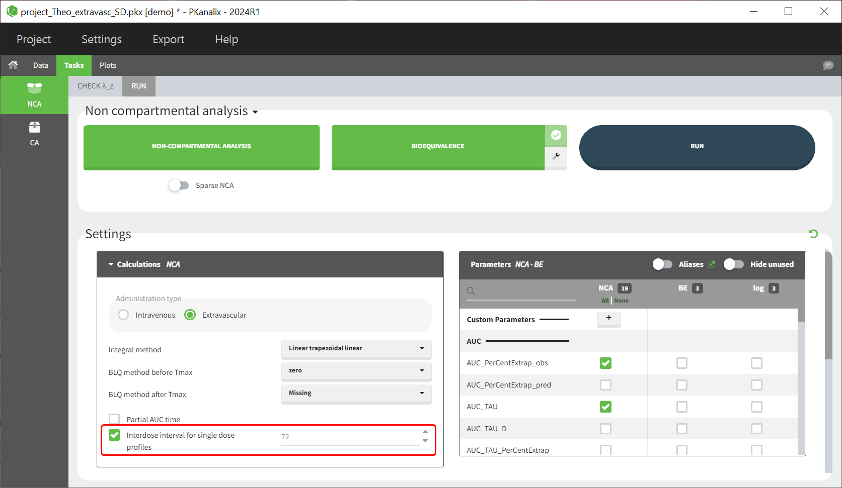
Single dose parameters are always calculated, irrespective of the presense or abscence of an inter-dose interval column in the dataset or whether the checkbox “Interdose interval for single dose profiles” is ticket or not.
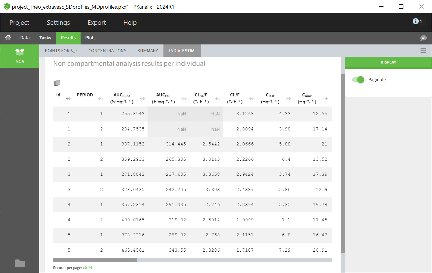
Steady-state parameters are calculated for all individuals if the checkbox “Interdose interval for single dose profiles” is ticked (and a value for tau is defined). They are also calculated for individuals having a positive interdose interval is defined in the dataset or if the profile (subject or occasion) contains several doses. Deepnding on the dataset, you may have some profiles with steady-state parameters and some without (appearing as NaN in the results).
Some parameters have identical names but are computed using different formulas, contingent upon whether it pertains to a single dose profile or a multiple dose profile:
| Name | Formula/Description – SD | Formula/Description – SS |
|---|---|---|
| C0 | Concentration at dosing time. If profile doesn’t contain obs at dosing time: Extravascular or Infusion: C0 = 0. For IV bolus: log-linear regression of first two data points to back-extrapolate C0. | Minimum observed during the dose interval. |
| Cmax | Maximum observed concentration, occurring at Tmax. If not unique, then the first maximum is used. | Maximum observed concentration between dose time and dose time + TAU. |
| Cmax_D | Cmax/Dose | Cmax (based on SS)/Dose |
| Tmax | Time of maximum observed concentration; entire curve is considered. | Tmax corresponds to points collected during a dosing interval. |
| MRTINF_obs | Intravascular: MRTINF_obs = AUMCINF_obs/AUCINF_obs – TI/2; TI
infusion duration Extravascular: MRTINF_obs = AUMCINF_obs/AUCINF_obs → AUMCINF_obs & AUCINF_obs based on Clast_obs. |
Mean Residence Time extrapolated to infinity using predicted Clast, calculated using AUC_TAU. |
| MRTINF_pred | Same formulas as above but based on AUMCINF_pred & AUCINF_pred based on Clast_pred. | |
| Vss_obs | Vss_obs=MRTINF_obs * Cl_obs with MRTINF_obs for SD profiles | Vss_obs=MRTINF_obs * Cl_obs with MRTINF_obs for SS profiles |
| Vss_pred | Vss_pred=MRTINF_pred * Cl_pred with MRTINF_pred for SD profiles | Vss_pred=MRTINF_pred * Cl_pred with MRTINF_pred for SS profiles |
These parameters are distinguished by the postfix “_SS” in the list of parameters and in the results table. This extension is also echoed in the aliases by the postfix “, SS”.
Typically, parameters that share the same name are calculated differently based on whether the “Interdose interval for single dose profiles” checkbox is selected. However, there’s one exception: parameter C0. In cases where both single dose and multiple dose profiles occur together, the order of profiles influences C0‘s calculation. If the first profile is a single dose, followed by either more single dose profiles or multiple dose profiles, and the checkbox is enabled, C0 for the first occasion follows the single dose formula, while subsequent C0‘s follow the steady-state formula.
Ratios for NCA parameters
Starting from PKanalix version 2024R1 and above, ratios for each individual of NCA metrics along occasions can now be calculated. In the dedicated section “Ratios NCA” in the NCA tasks tab, ratios can be defined by clicking on the plus sign (red frame). This action prompts a window to appear, allowing you to specify the ratio in greater detail.
The ratio is calculated for each individual, using the different occasions (i.e profiles). When only one occasion corresponds to the modality selected for “ref” and “test”, the ratio is simply the ratio of the two values. If there are subjects who have multiple occasions corresponding to the modality selected for “ref” and “for “test”, the arithmetic mean of the values for this modality is calculated first, then the ratio is calculated.
If there are subjects without a parameter value for one of the test or comparison modalities, no ratio can be calculated for this parameter. Consequently, the subject obtains NaN as a result.