In PKanalix, a dataset should be loaded in the Data tab to create a project. Once the dataset accepted, it is possible to specify units and filter the dataset, so units and filtering information should not be included in the file loaded in the Data tab.
The data set format used in PKanalix is the same as for the entire MonolixSuite, to allow smooth transitions between applications. In this format:
- Each line corresponds to one individual and one time point.
- Each line can include a single measurement (also called observation), or a dose amount (or both a measurement and a dose amount).
- Dosing information should be indicated for each individual in a specific column, even if it is the same treatment for all individuals.
- Headers are free but there can be only one header line.
- Different types of information (dose, observation, covariate, etc) are recorded in different columns, which must be tagged with a column type (see below).
If your dataset is not in this format, in most cases, it is possible to format it in a few steps in the data formatting tab, to incorporate the missing information.
- Overview of most common column types
- Example datasets
- Plasma concentration data
- Steady-state data
- BLQ data
- Urine data
- Occasions (“Sort” variables)
- Covariates (“Carry” variables)
- Other useful column-types
- Description of all possible column types
Overview of most common column-types
A data set typically contains only the following columns: ID (mandatory), TIME (mandatory), OBSERVATION (mandatiry), AMOUNT (optional). The main rules for interpreting the dataset are:
- Cells that do not contain information (e.g AMOUNT column on a line recording a measurement) should have a dot.
- Headers are free but there can be only one header line and the columns must be assigned to one of the available column-types. The full list of column-types is available at the end of this page and a detailed description is given on the dataset documentation website.
The most common column types in addition to ID, TIME, OBSERVATION and AMOUNT are:
- For IV infusion data, an additional INFUSION RATE or INFUSION DURATION is necessary.
- For steady-state data, either an INTERDOSE INTERVAL column is added, or the interdose interval tau is specified in the NCA settings.
- If a dose and a measurement occur at the same time, they can be encoded on the same line or on different lines.
- Sort and carry variables can be defined using the OCCASION, and CATEGORICAL COVARIATE and CONTINUOUS COVARIATE column-types.
- BLQ data are defined using the CENSORING and LIMIT column-types.
In addition to the typical cases presented above, a few additional column-types may also be convenient:
- ignoring a line: with the IGNORED OBSERVATION (ignores the measurement only) or IGNORED LINE (ignores the entire line, including regressor and dose information). However it is more convenient to filter lines of your dataset without modifying it by using filters (available once your dataset is accepted).
- working with several types of observations: If several observation types are present in the dataset (for example parent and metabolite), all measurements should still appear in the same OBSERVATION column, and another column should be used to distinguish the observation types. If this is not the case in your dataset, data formatting enables to merge several observation columns. To run NCA for several observations at the same time for the same id, tag the column listing the observation types as OCCASION . To run CA for several observations with a model including several outputs (for example PK and PD), tag the column listing the observation types as OBSERVATION ID. In this case, only one observation type will be available for NCA. It can be selected in the “NCA” section to perform the calculations.
- working with several types of administrations: a single data set can contain different types of administrations, for instance IV bolus and extravascular, distinguished using the ADMINISTRATION ID column-type. The setting “administration type” in “Tasks>Run” can be chosen separately for each administration id, and the appropriate parameter calculations will be performed.
Example datasets
Below we show how to encode the dataset for most typical situations.
Plasma concentration data
Extravascular
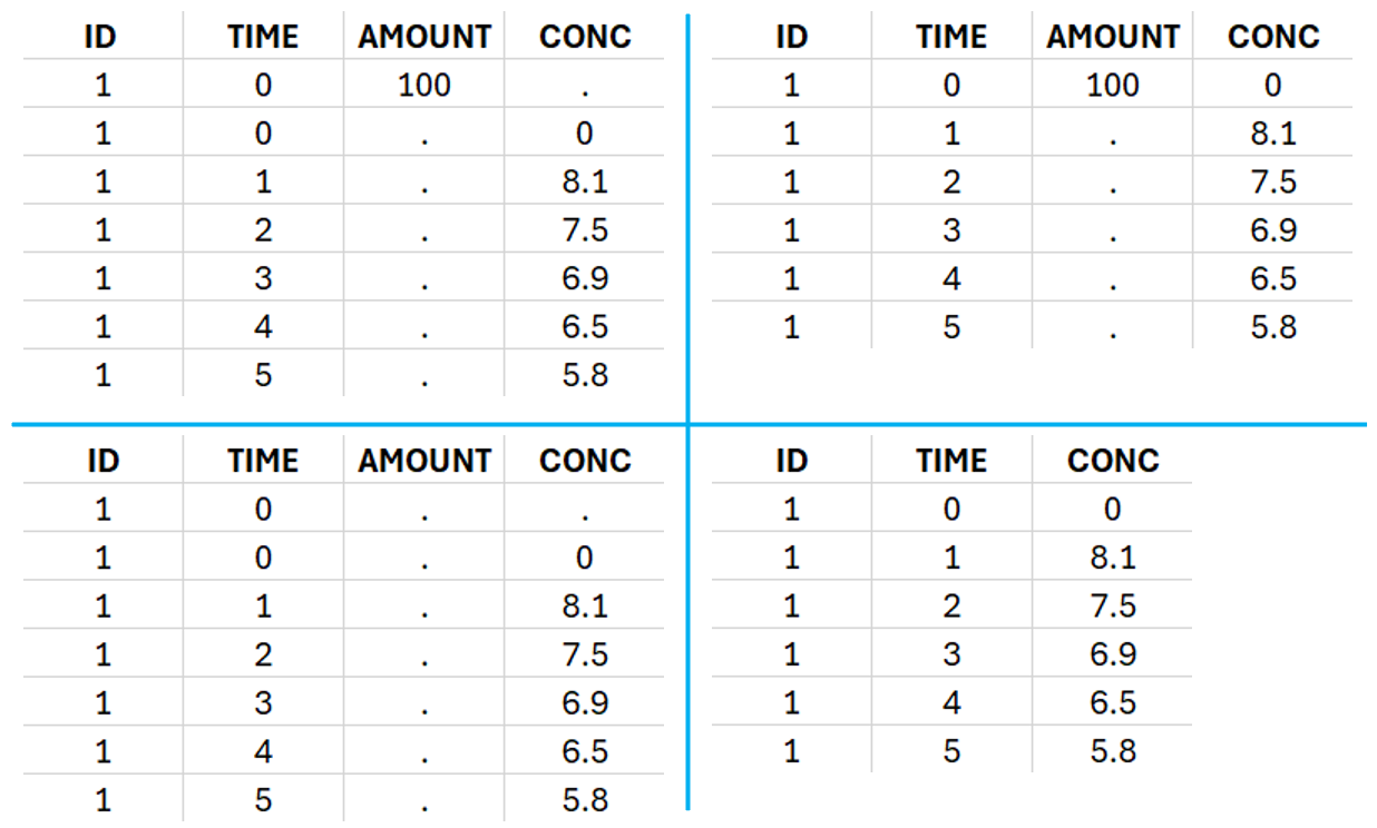
For extravascular administration, the mandatory column-types are ID (individual identifiers as integers or strings), OBSERVATION (measured concentrations), AMOUNT (dose amount administered, mandatory for 2023 and previous versions) and TIME (time of dose or measurement). Since version 2024, datasets that do not contain an AMOUNT column or no information in the AMOUT column are accepted for single dose or multiple dose administrations.
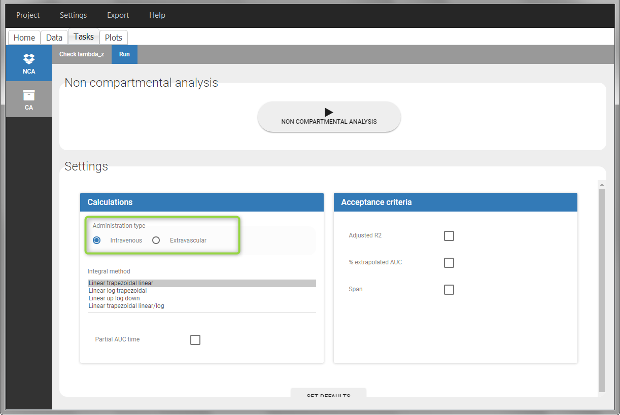
To distinguish the extravascular from the IV bolus case, in “Tasks>Run” the administration type must be set to “extravascular”.
If no measurement is recorded at the time of the dose, a concentration of zero is added for single dose data, the minimum concentration observed during the dose interval for steady-state data.
Example:
- demo project_extravascular.pkx
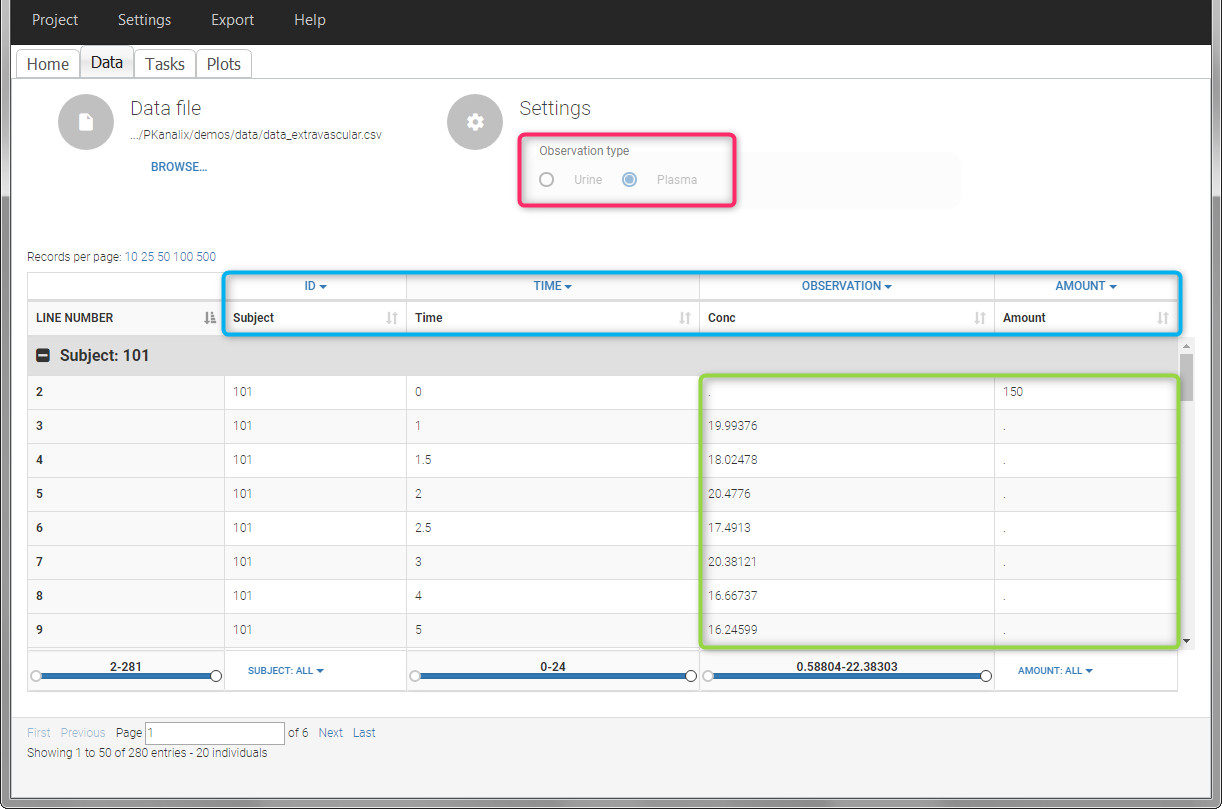
This data set records the drug concentration measured after single oral administration of 150 mg of drug in 20 patients. For each individual, the first line records the dose (in the “Amount” column tagged as AMOUNT column-type) while the following lines record the measured concentrations (in the “Conc” column tagged as OBSERVATION). Cells of the “Amount” column on measurement lines contain a dot, and respectively for the concentration column. The column containing the times of measurements or doses is tagged as TIME column-type and the subject identifiers, which we will use as sort variable, are tagged as ID. Check the OCCASION section if more sort variables are needed. After accepting the dataset, the data is automatically assigned as “Plasma”.
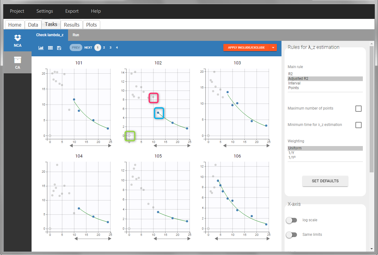
In the “Tasks/Run” tab, the user must indicate that this is extravascular data. In the “Check lambda_z”, on linear scale for the y-axis, measurements originally present in the data are shown with full circles. Added data points, such as a zero concentration at the dose time, are represented with empty circles. Points included in the \(\lambda_z\) calculation are highlighted in blue.
 |
 |
After running the NCA analysis, PK parameters relevant to extravascular administration are displayed in the “Results” tab.
IV infusion
Intravenous infusions are indicated in the data set via the presence of an INFUSION RATE or INFUSION DURATION column-type, in addition to the ID (individual identifiers as integers or strings), OBSERVATION (measured concentrations), AMOUNT (dose amount administered, mandatory for 2023 and previous versions) and TIME (time of dose or measurement). The infusion duration (or rate) can be identical or different between individuals. Since version 2024, datasets that do not contain an AMOUNT column or no information in the AMOUT column are accepted for single dose or multiple dose administrations.
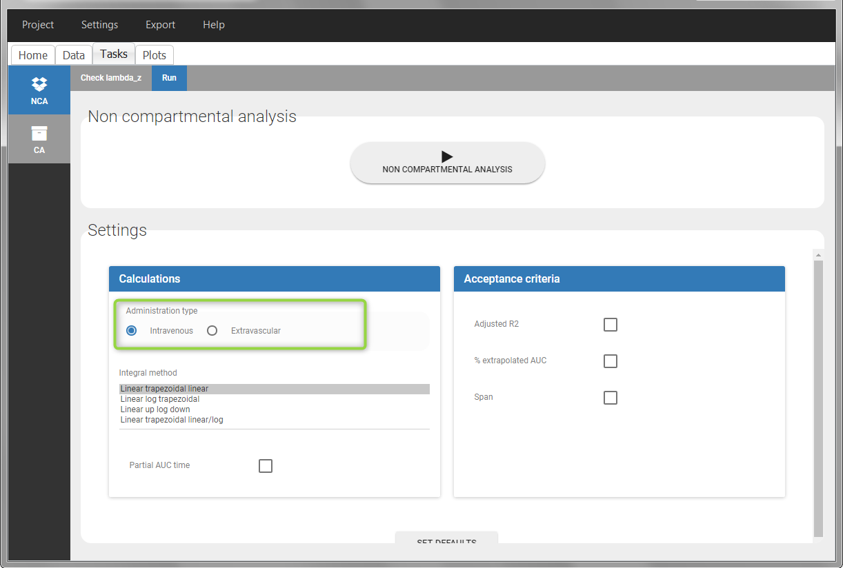
In “Tasks>Run” the administration type must be set to “intravenous”.
If no measurement is recorded at the time of the dose, a concentration of zero is added for single dose data, the minimum concentration observed during the dose interval for steady-state data.
Example:
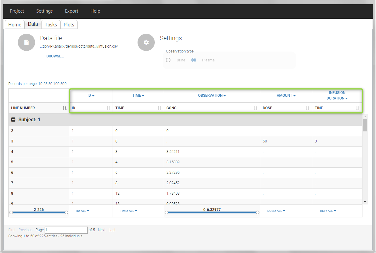
- demo project_ivinfusion.pkx:
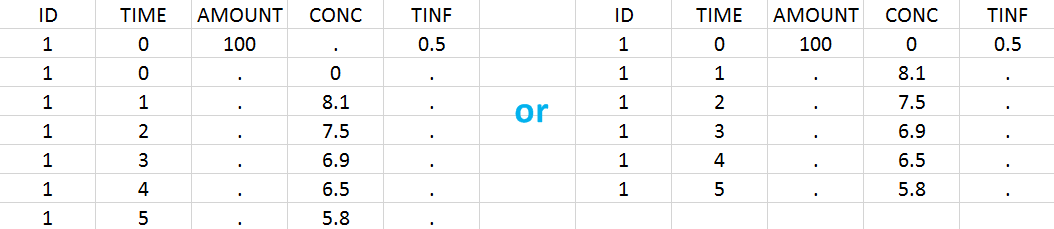
In this example, the patients receive an iv infusion over 3 hours. The infusion duration is recorded in the column called “TINF” in this example, and tagged as INFUSION DURATION.
In the “Tasks/Run” tab, the user must indicate that this is intravenous data.
IV bolus
For IV bolus administration, the mandatory column-types are ID (individual identifiers as integers or strings), OBSERVATION (measured concentrations), AMOUNT (dose amount administered, mandatory for 2023 and previous versions) and TIME (time of dose or measurement). Since version 2024, datasets that do not contain an AMOUNT column or no information in the AMOUT column are accepted for single dose or multiple dose administrations.
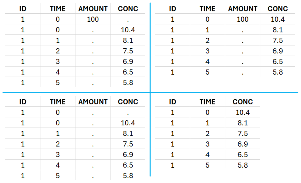
To distinguish the IV bolus from the extravascular case, in “Tasks>Run” the administration type must be set to “intravenous”.
If no measurement is recorded at the time of the dose, the concentration of at time zero is extrapolated using a log-linear regression of the first two data points, or is taken to be the first observed measurement if the regression yields a slope >= 0. See the calculation details for more information.
Example:
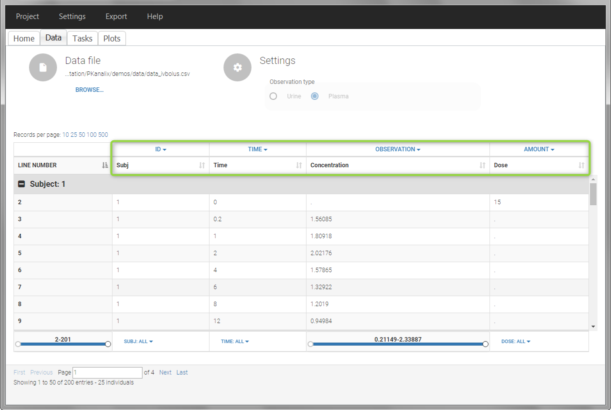
- demo project_ivbolus.pkx:
In this data set, 25 individuals have received an iv bolus and their plasma concentration have been recorded over 12 hours. For each individual (indicated in the column “Subj” tagged as ID column-type), we record the dose amount in a column “Dose”, tagged as AMOUNT column-type. The measured concentrations are tagged as OBSERVATION and the times as TIME. Check the OCCASION section if more sort variables are needed in addition to ID. After accepting the dataset, the data is automatically assigned as “plasma”.
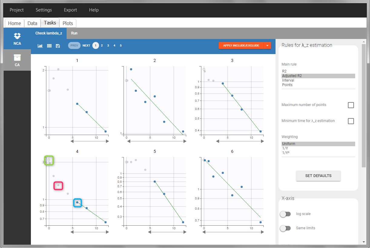
In the “Tasks/Run” tab, the user must indicate that this is intravenous data. In the “Check lambda_z”, measurements originally present in the data are shown with full circles. Added data points, such as the C0 at the dose time, are represented with empty circles. Points included in the \(\lambda_z\) calculation are highlighted in blue.
 |
 |
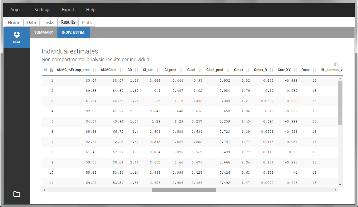
After running the NCA analysis, PK parameters relevant to iv bolus administration are displayed in the “Results” tab.
Steady-state
Starting from version 2024, the interdose interval tau used to calculate NCA parameters specific to steady-state can be specified either in the dataset column tagged as INTERDOSE INTERVAL, or directly as part of the NCA settings.
In the 2023 and previous versions, it was necessary to indicate steady-state using the STEADY STATE column-type: SS=1 indicates that the individual is already at steady-state when receiving the dose. This implicitly assumes that the individual has received many doses before this one. SS=0 or ‘.’ indicates a single dose. Starting from version 2024, the SS column is accepted but not mandatory anymore.
The dosing interval (also called tau) is indicated in the INTERDOSE INTERVAL column on the lines defining the doses, or as part of the NCA settings.
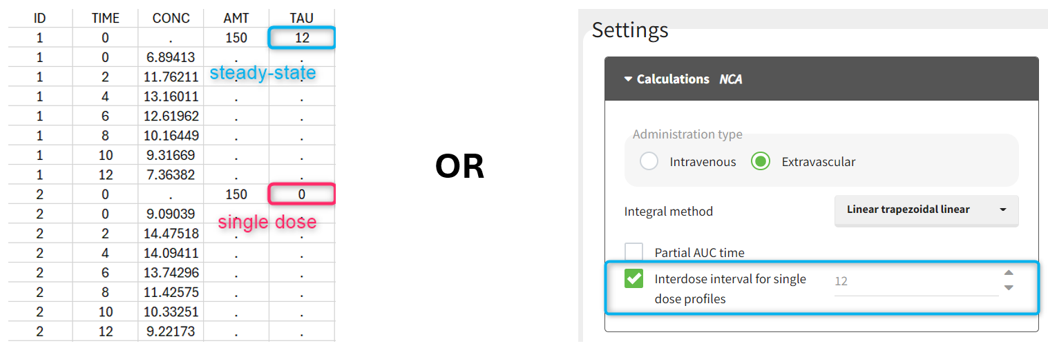
Steady state calculation formulas will be applied for individuals having a dose with INTERDOSE INTERVAL = double. A data set can contain individuals which are at steady-state and some which are not. If the NCA setting “Interdose interval for single dose profiles” is selected, steady-state parameters are calculated for all individuals.
If no measurement is recorded at the time of the dose, the minimum concentration observed during the dose interval is added at the time of the dose for extravascular and infusion data. For iv bolus, a regression using the two first data points is performed. Only measurements between the dose time and dose time + interdose interval will be used.
Examples:
- demo project_steadystate.pkx:
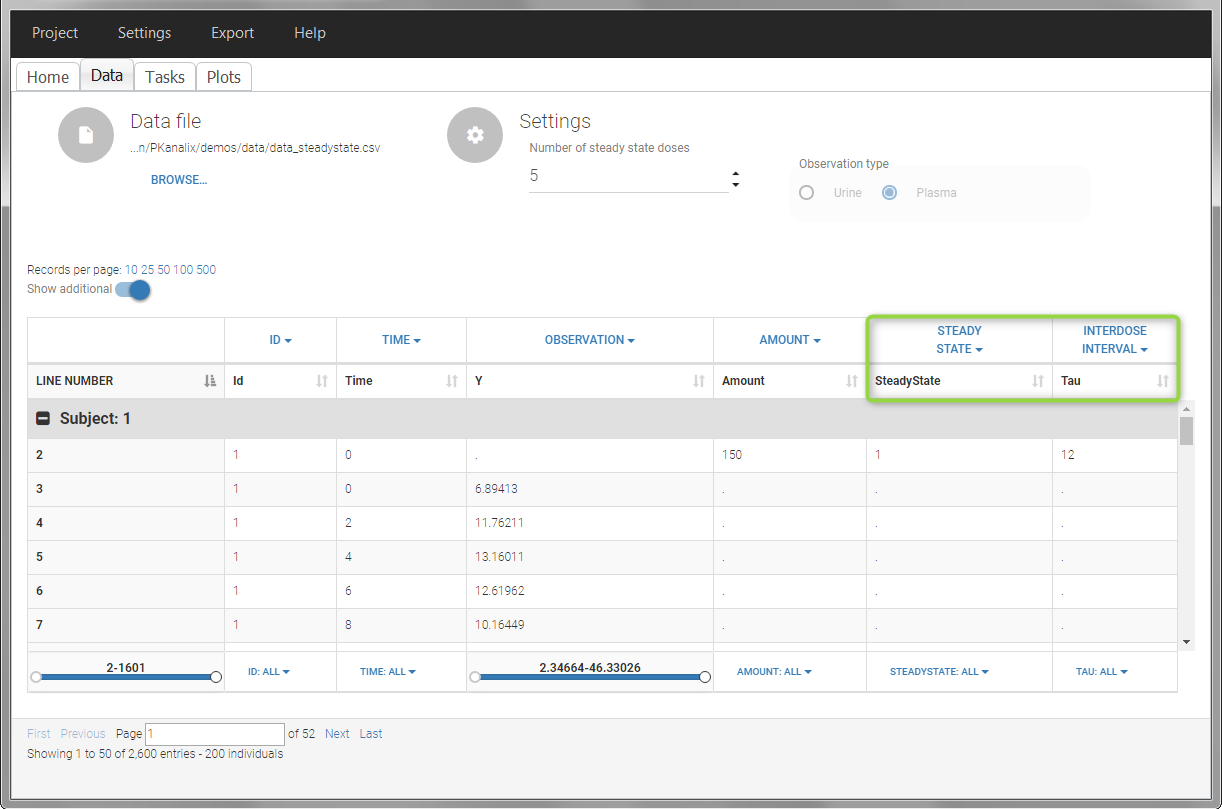
In this example, the individuals are already at steady-state when they receive the dose. This is indicated in the data set via the column “SteadyState” tagged as STEADY STATE column-type, which contains a “1” on lines recording doses. The interdose interval is noted on those same line in the column “tau” tagged as INTERDOSE INTERVAL. When accepting the data set, a “Settings” section appears, which allows to define the number of steady-state doses. This information is relevant when exporting to Monolix, but not used in PKanalix directly.
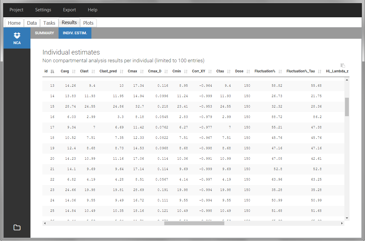
After running the NCA estimation task, steady-state specific parameters are displayed in the “Results” tab.
BLQ data
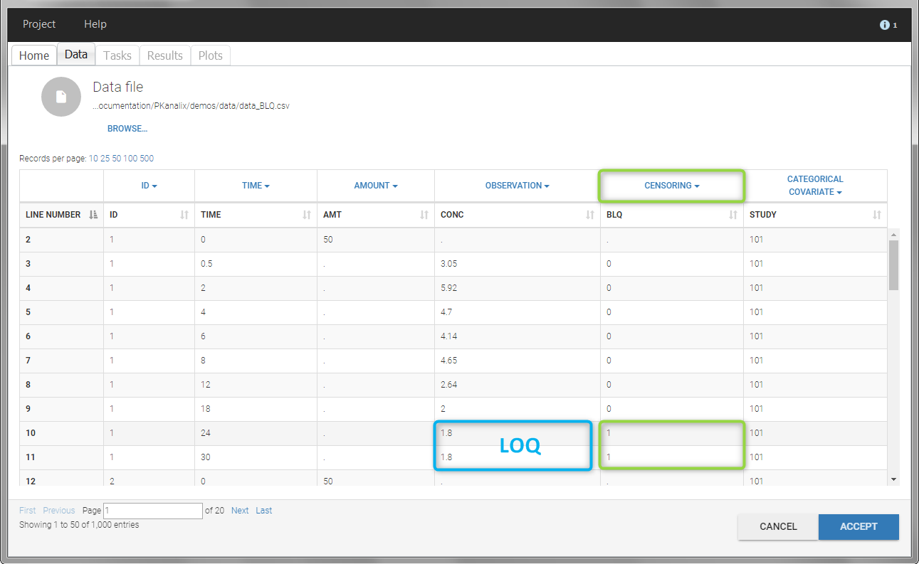
Below the limit of quantification (BLQ) data can be recorded in the data set using the CENSORING column:
- “0” indicates that the value in the OBSERVATION column is the measurement.
- “1” indicates that the observation is BLQ.
The lower limit of quantification (LOQ) must be indicated in the OBSERVATION column when CENSORING = “1”. Note that strings are not allowed in the OBSERVATION column (except dots). A different LOQ value can be used for each BLQ data.
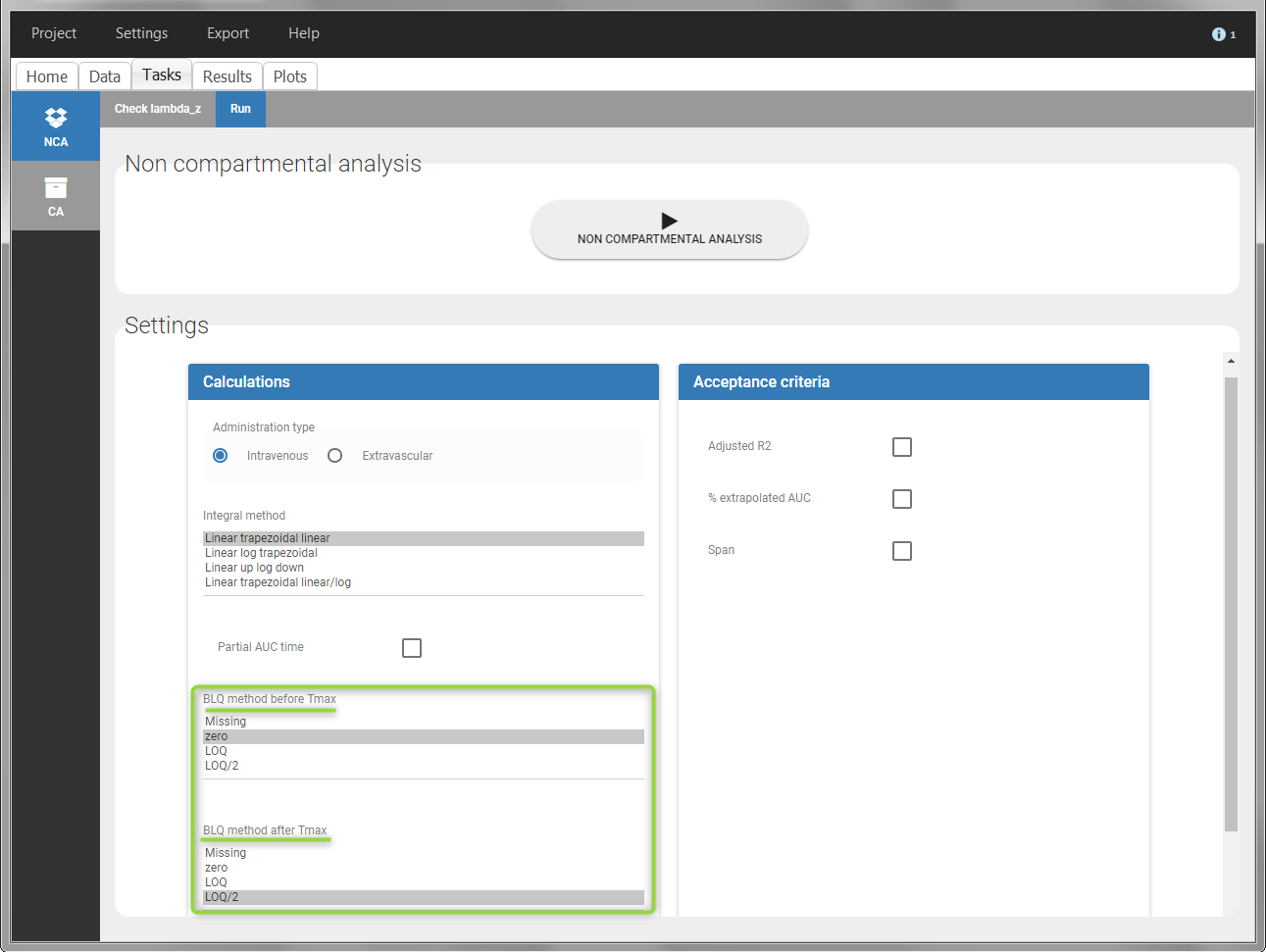
When performing an NCA analysis, the BLQ data before and after the Tmax are distinguished. They can be replaced by:
- zero
- the LOQ value
- the LOQ value divided by 2
- or considered as missing
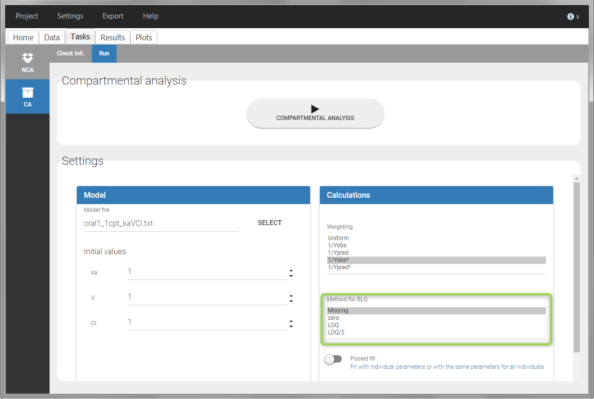
For a CA analysis, the same options are available, but no distinction is done between before and after Tmax. Once replaced, the BLQ data are handled as any other observation.
A LIMIT column can be added to record the other limit of the interval (in general zero). This value will not be used by PKanalix but can facilitate the transition from an NCA/CA analysis PKanalix to a population model with Monolix.
To easily encode BLQ data in a dataset that only has BLQ tags in the observation column, you can use Data formatting.
Examples:
- demo project_censoring.pkx: two studies with BLQ data with two different LOQ
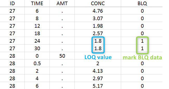
In this dataset, the measurements of two different studies (indicated in the STUDY column, tagged as CATEGORICAL COVARIATE in order to be carried over) are recorded. For the study 101, the LOQ is 1.8 ug/mL, while it is 1 ug/mL for study 102. The BLQ data are marked with a “1” in the BLQ column, which is tagged as CENSORING. The LOQ values are indicated for each BLQ in the CONC column of measurements, tagged as OBSERVATION.
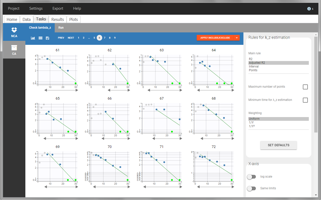
In the “Task>NCA>Run” tab, the user can choose how to handle the BLQ data. For the BLQ data before and after the Tmax, the BLQ data can be considered as missing (as if this data set row would not exist), or replaced by zero (default before Tmax), the LOQ value or the LOQ value divided by 2 (default after Tmax). In the “Check lambda_z” tab, the BLQ data are shown in green and displayed according to the replacement value.
 |
 |
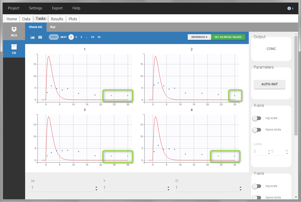
For the CA analysis, the replacement value for all BLQ can be chosen in the settings of the “Run” tab (default is Missing). In the “Check init.” tab, the BLQ are again displayed in green, at the LOQ value (irrespective of the chosen method for the calculations).
 |
 |
Urine data
To work with urine data, it is necessary to record the time and amount administered, the volume of urine collected for each time interval, the start and end time of the intervals and the drug concentration in a urine sample of each interval. The time intervals must be continuous (no gaps allowed).
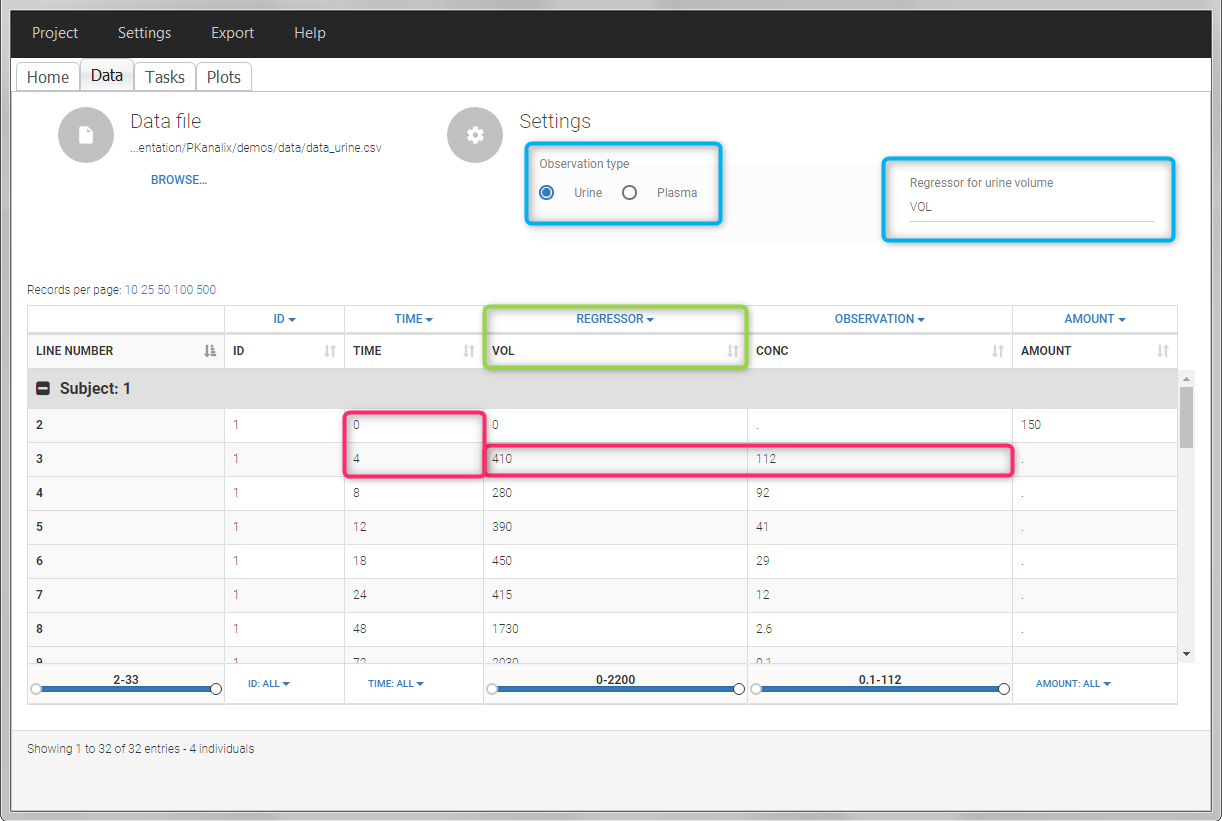
In PKanalix, the start and end times of the intervals are recorded in a single column, tagged as TIME column-type. In this way, the end time of an interval automatically acts as start time for the next interval. The concentrations are recorded in the OBSERVATION column. The volume column must be tagged as REGRESSOR column type. This general column-type of MonolixSuite data sets allows to easily transition to the other applications of the Suite. As several REGRESSOR columns are allowed, the user can select which REGRESSOR column should be used as volume. The concentration and volume measured for the interval [t1,t2] are noted on the t2 line. The volume value on the dose line is meaningless, but it cannot be a dot. We thus recommend to set it to zero.
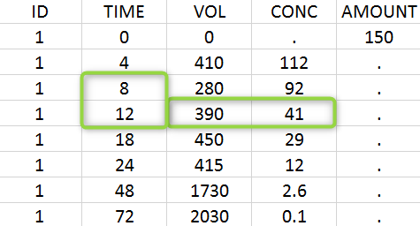
A typical urine data set has the following structure. A dose of 150 ng has been administered at time 0. The first sampling interval spans from the dose at time 0 to 4h post-dose. During this time, 410 mL of urine have been collected. In this sample, the drug concentration is 112 ng/mL. The second interval spans from 4h to 8h, the collected urine volume is 280 mL and its concentration is 92 ng/mL. The third interval is marked on the figure: 390mL of uring have been collected from 8h to 12h.
The given data is used to calculate the intervals midpoints, and the excretion rates for each interval. This information is then used to calculate the \(\lambda_z\) and calculate urine-specific parameters. In “Tasks/Check lambda_z”, we display the midpoints and excretion rates. However, in the “Plots>Data viewer”, we display the measured concentrations at the end time of the interval.
Example:
- demo project_urine.pkx: urine PK dataset
In this urine PK data set, we record the consecutive time intervals in the “TIME” column tagged as TIME. The collected volumes and measured concentration are in the columns “VOL” and “CONC”, respectively tagged as REGRESSOR and OBSERVATION. Note that the volume and concentration are indicated on the line of the interval end time. The volume on the first line (start time of the first interval, as well as dose line) is set to zero as it must be a double. This value will not be used in the calculations. Once the dataset is accepted, the observation type must be set to “urine” and the regressor column corresponding to the volume defined.
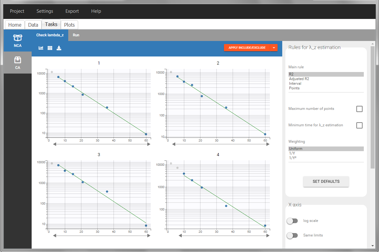
In “Tasks>Check lambda_z”, the excretion rate are plotted on the midpoints time for each individual. The choice of the lambda_z works as usual.
Once the NCA task has run, urine-specific PK parameters are displayed in the “Results” tab.

Occasions (“Sort” variables)
The main sort level are the individuals indicated in the ID column. Additional sort levels can be encoded using one or several OCCASION column(s). OCCASION columns contain integer values that permit to distinguish different time periods for a given individual. The time values can restart at zero or continue when switching from one occasion to the next one. The variables differing between periods, such as the treatment for a crossover study, are tagged as CATEGORICAL or CONTINUOUS COVARIATES (see below). The NCA and CA calculations will be performed on each ID-OCCASION combination. Each occasion is considered independent of the other occasions (i.e a washout is applied between each occasion).
Note: occasions columns encoding the sort variables as integers can easily be added to an existing data set using Excel or R.
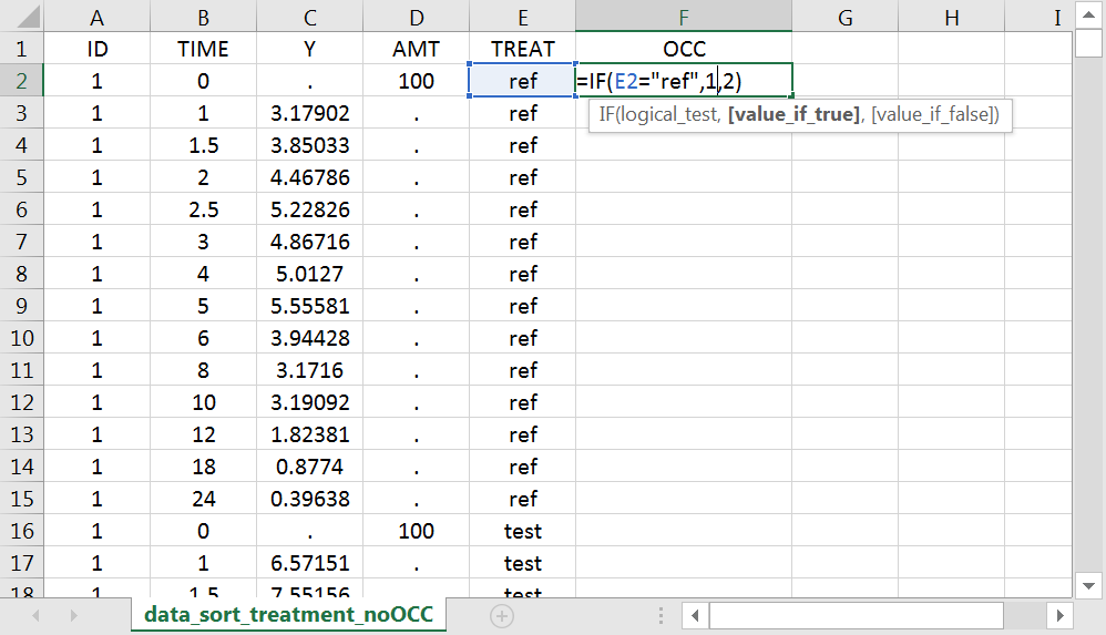
With R, the “OCC” column can be added to an existing “data” data frame with a column “TREAT” using data$OCC <- ifelse(data$TREAT=="ref", 1, 2).
With Excel, assuming the sort variable is encoded in the column E with values “ref” and “test”, type =IF(E2="ref",1,2) to generate the first value of the “OCC” column and then propagate to the entire column:
Examples:
- demo project_occasions1.pkx: crossover study with two treatments
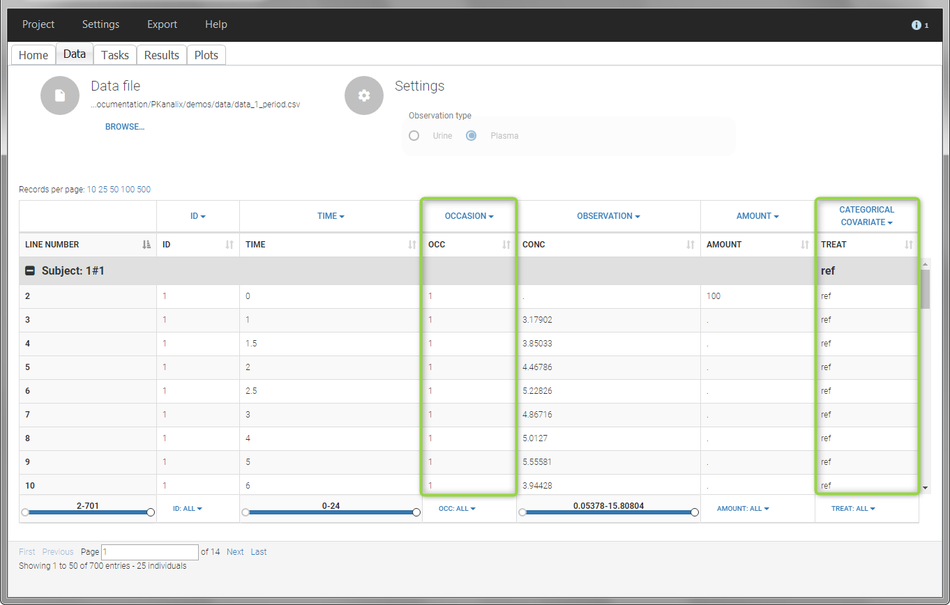
The subject column is tagged as ID, the treatment column as CATEGORICAL COVARIATE and an additional column encoding the two periods with integers “1” and “2” as OCCASION column.
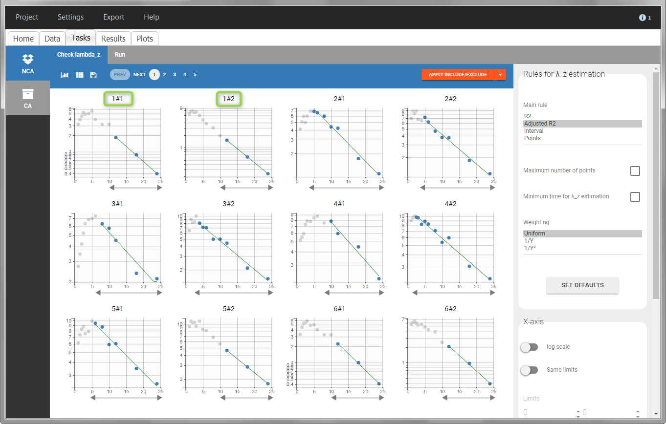
In the “Check lambda_z” (for the NCA) and the “Check init.” (for CA), each occasion of each individual is displayed. The syntax “1#2” indicates individual 1, occasion 2, according to the values defined in the ID and OCCASION columns.
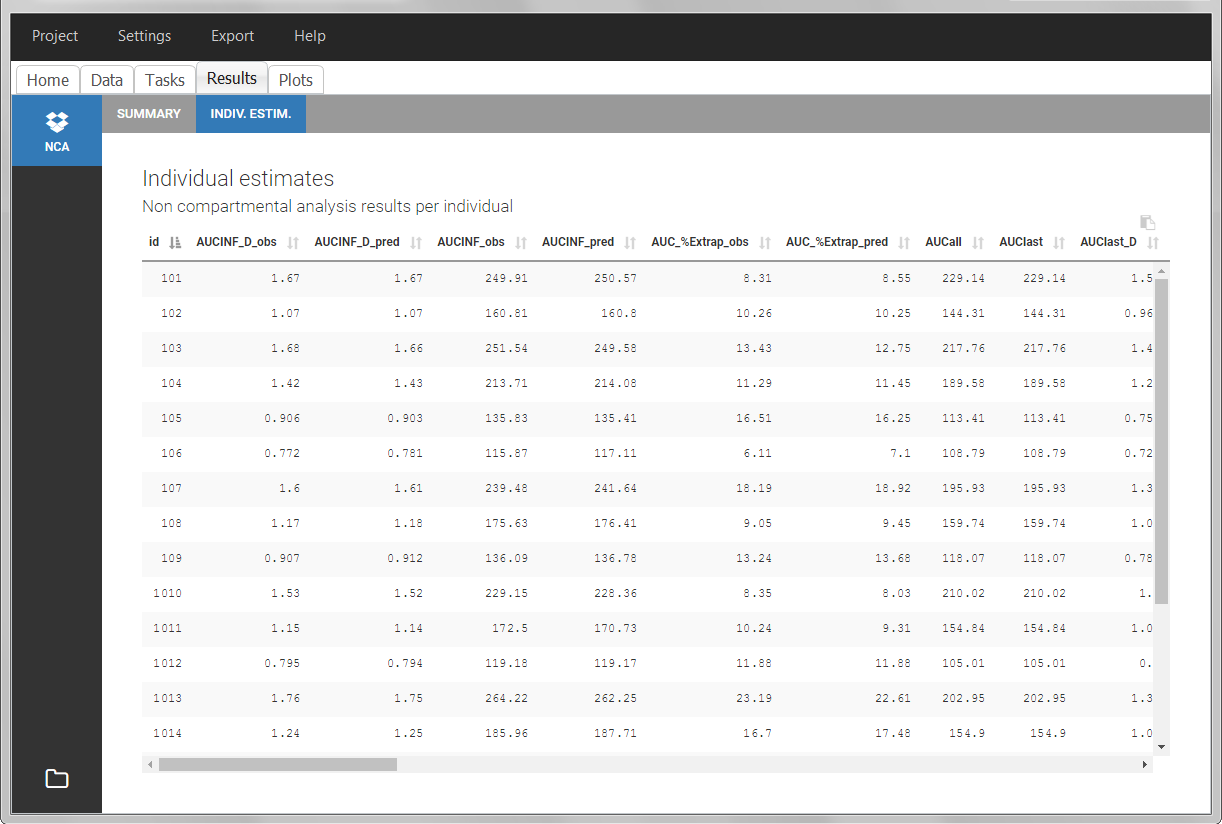
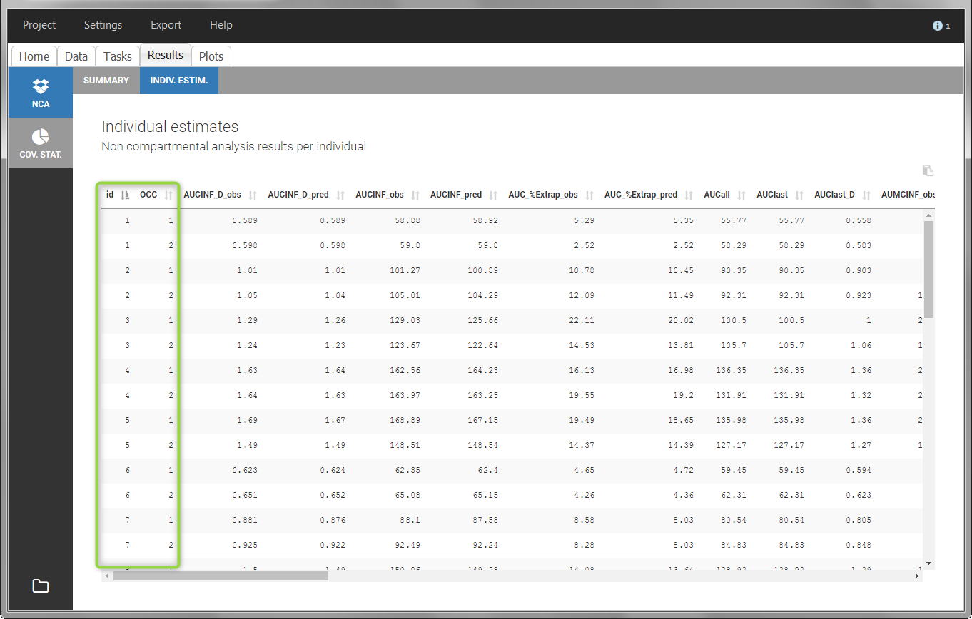
In the “Individual estimates” output tables, the first columns indicate the ID and OCCASION (reusing the data set headers). The covariates are indicated at the end of the table. Note that it is possible to sort the table by any column, including, ID, OCCASION and COVARIATES.
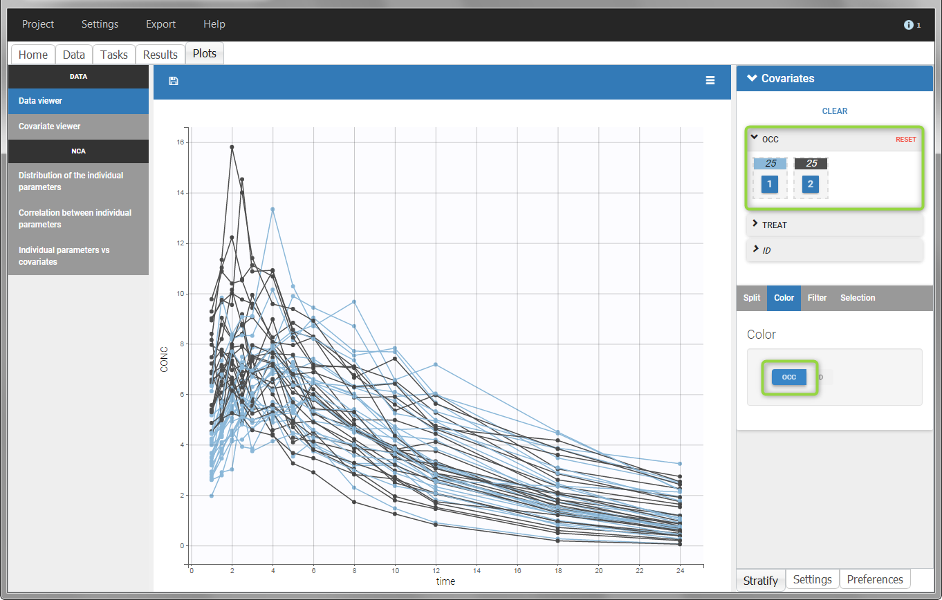
The OCCASION values are available in the plots for stratification, in addition to possible CATEGORICAL or CONTINUOUS COVARIATES (here “TREAT”).
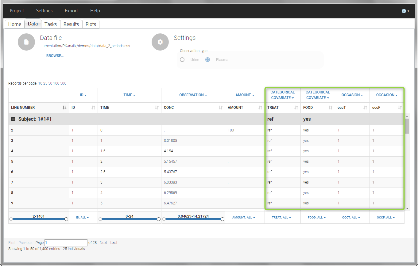
- demo project_occasions2.pkx: study with two treatments and with/without food
In this example, we have three sorting variables: ID, TREAT and FOOD. The TREAT and FOOD columns are duplicated: once with strings to be used as CATEGORICAL COVARIATE (TREAT and FOOD) and once with integers to be used as OCCASION (occT and occF).
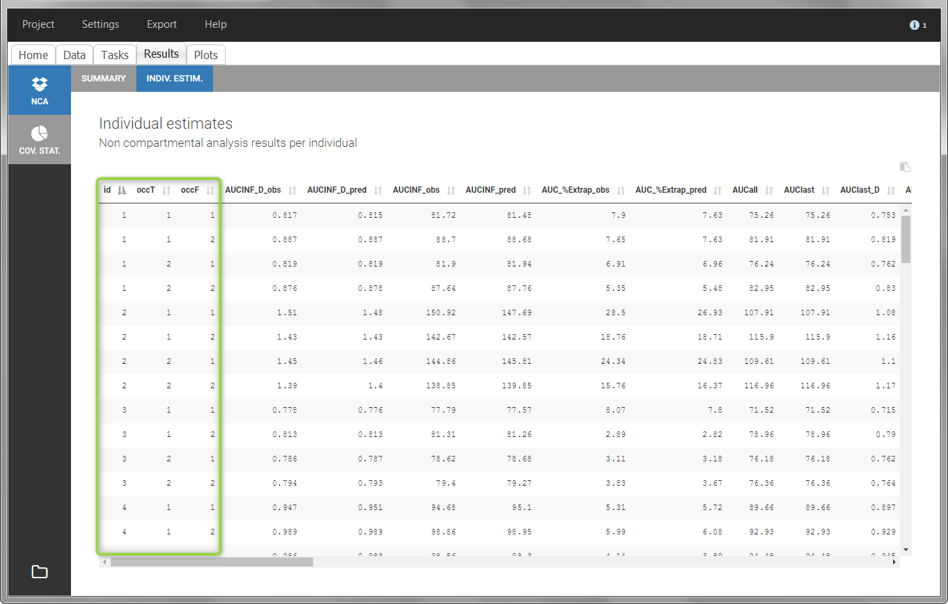
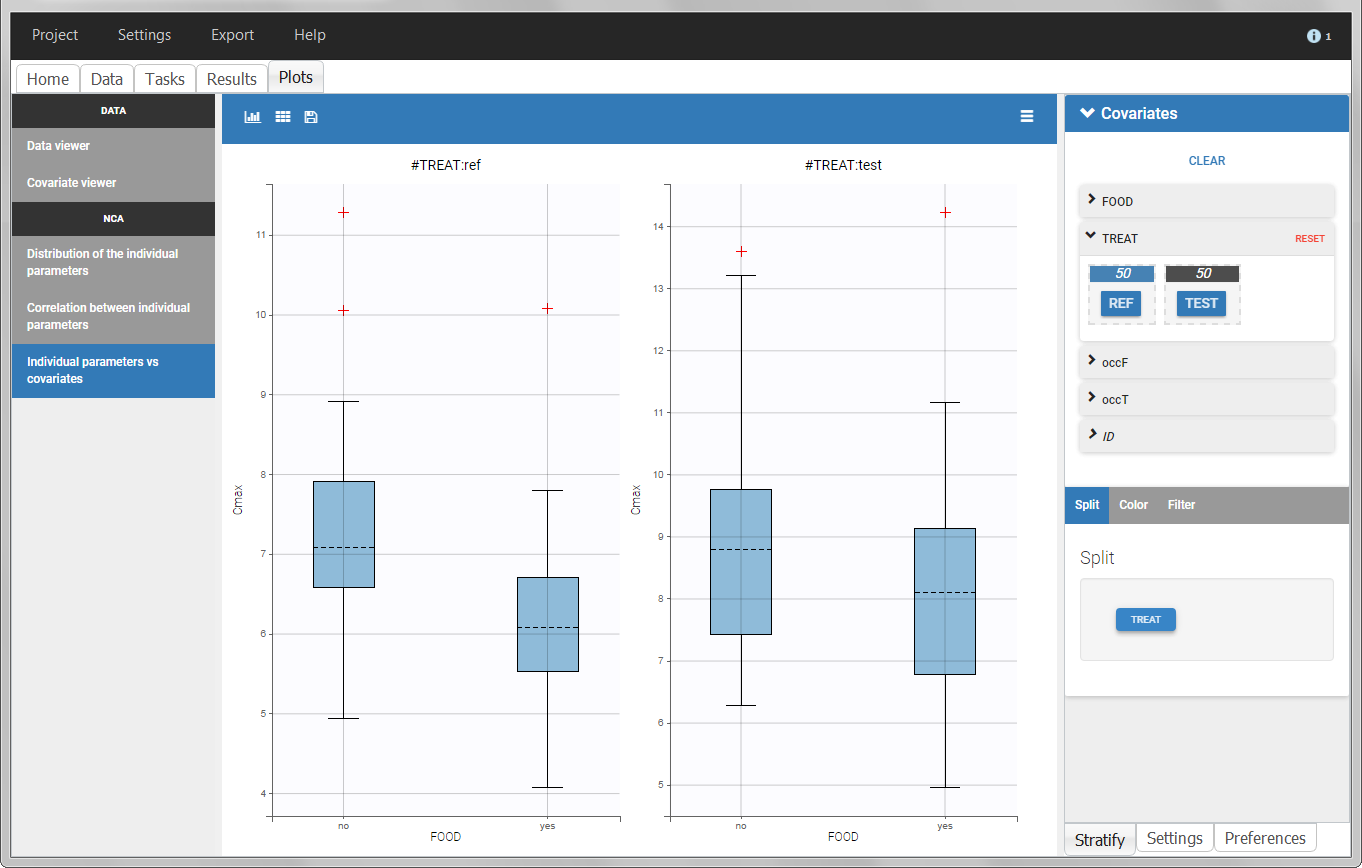
In the individual parameters tables and plots, three levels are visible. In the “Individual parameters vs covariates”, we can plot Cmax versus FOOD, split by TREAT for instance (Cmax versus TREAT split by FOOD is also possible).
 |
 |
Covariates (“Carry” variables)
Individual information that need to be carried over to output tables and plots must be tagged as CATEGORICAL or CONTINUOUS COVARIATES. Categorical covariates define variables with a few categories, such as treatment or sex, and are encoded as strings. Continuous covariates define variables on a continuous scale, such as weight or age, and are encoded as numbers. Covariates will not automatically be used as “Sort” variables. A dedicated OCCASION column is necessary (see above).
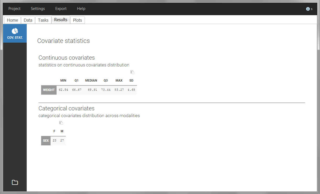
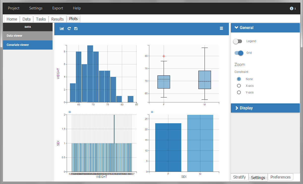
Covariates will automatically appear in the output tables. Plots of estimated NCA and/or CA parameters versus covariate values will also be generated. In addition, covariates can be used to stratify (split, color or filter) any plot. Statistics about the covariates distributions are available in table format in “Results > Cov. stat.” and in graphical format in “Plots > Covariate viewer”.
Note: It is preferable to avoid spaces and special characters (stars, etc) in the strings for the categories of the categorical covariates. Underscores are allowed.
Example:
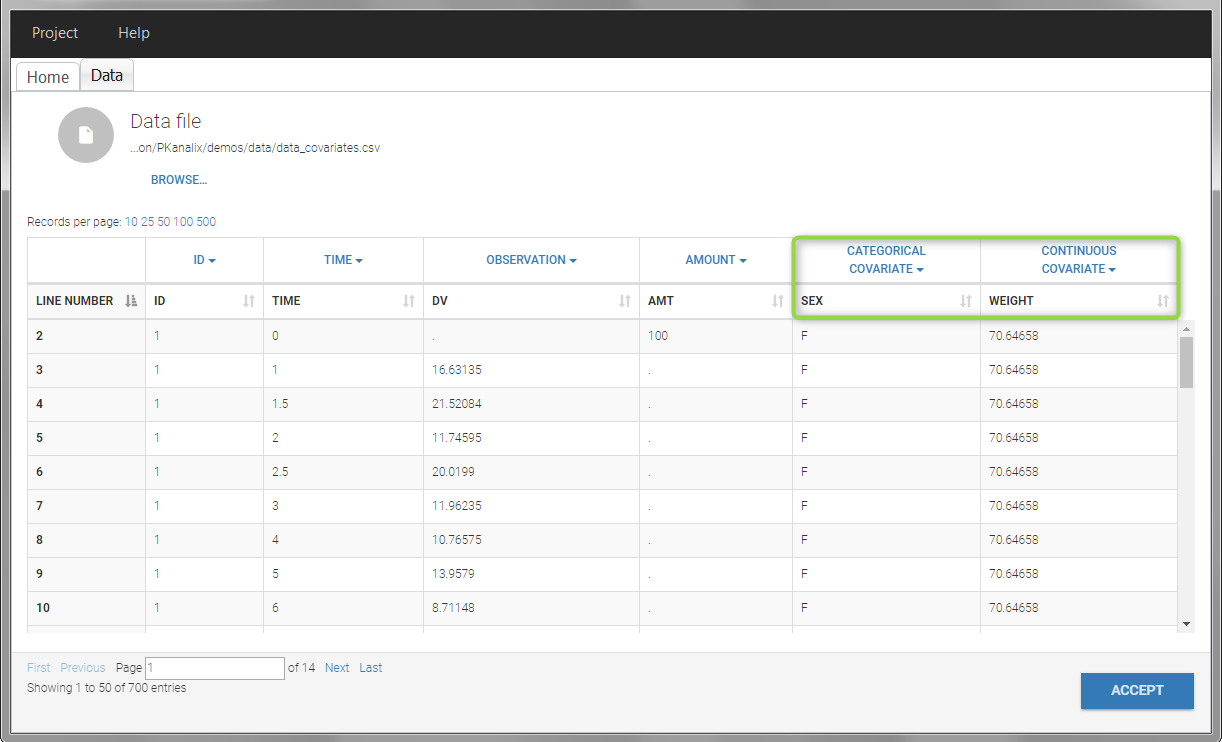
- demo project_covariates.pkx
In this data set, “SEX” is tagged as CATEGORICAL COVARIATE and “WEIGHT” as CONTINUOUS COVARIATE.
The “cov stat” table permits to see a few statistics of the covariate values in the data set. In the plot “Covariate viewer”, we see that the distribution of weight is similar for males and females.
 |
 |
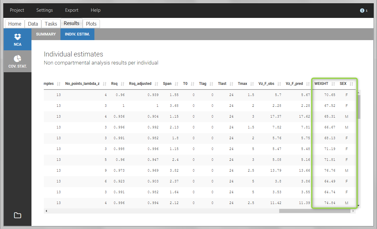
After running the NCA and CA tasks, both covariates appear in the table of individual estimated parameters estimated.
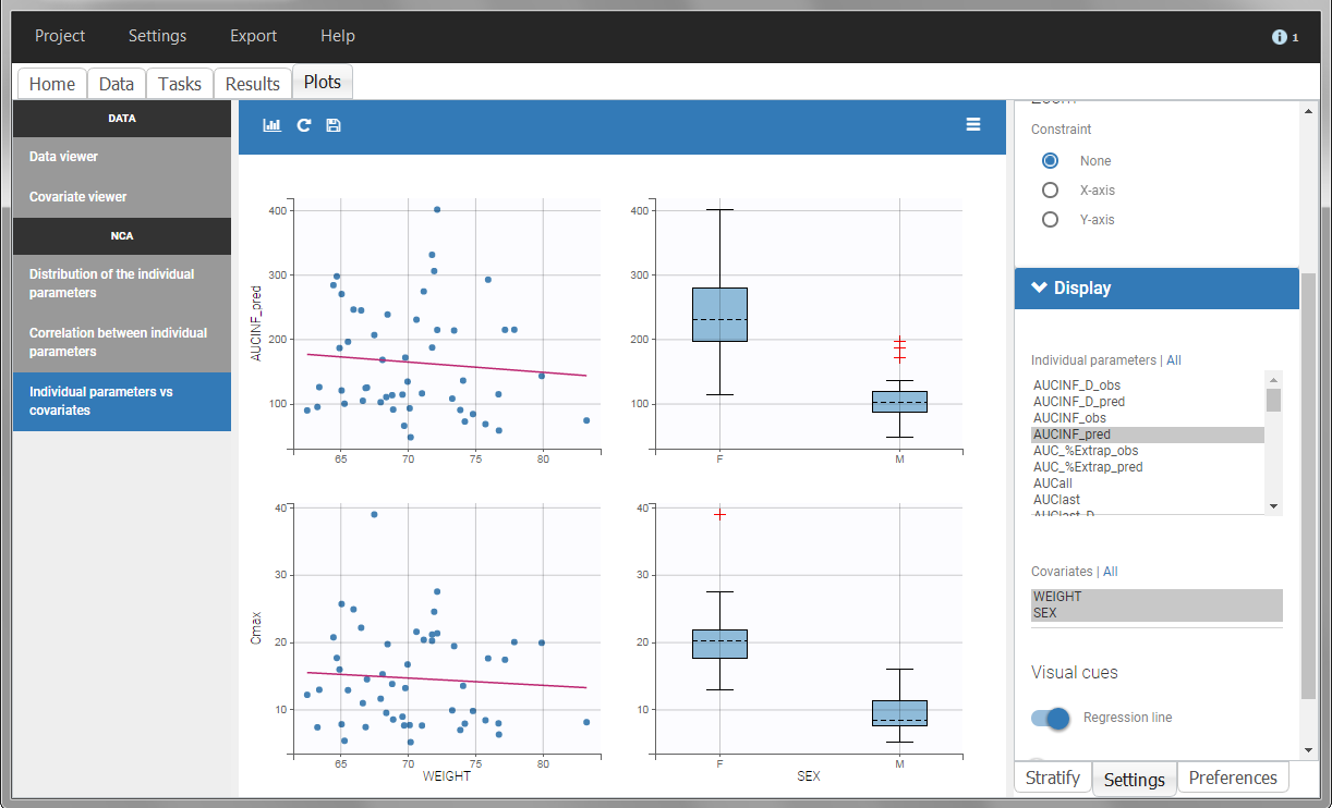
In the plot “parameters versus covariates”, the parameters values are plotted as scatter plot with the parameter value (here Cmax and AUCINF_pred) on on y-axis and the weight value on the x-axis, and as boxplots for sex female and sex male.
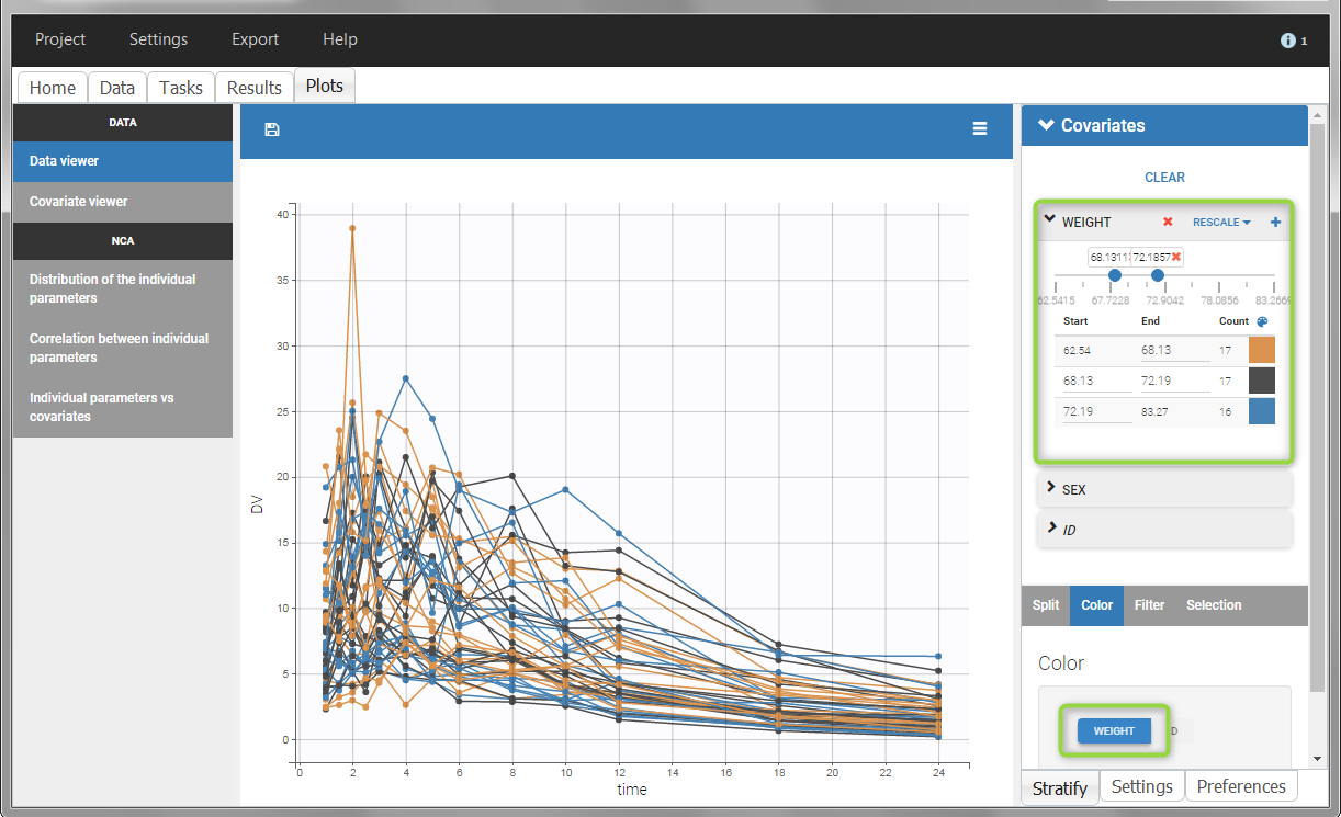
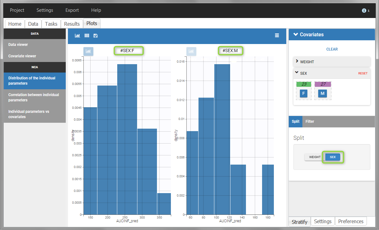
All plots can be stratified using the covariates. For instance, the “Data viewer” can be colored by weight after having created 3 weight groups. Below we also show the plot “Distribution of the parameters” split by sex with selection of the AUCINF_pred parameter.
 |
 |
Description of all possible column types
Column-types used for all types of lines:
- ID (mandatory): identifier of the individual
- OCCASION (formerly OCC): identifier (index) of the occasion
- TIME (mandatory): time of the dose or observation record
- NOMINAL TIME: time at which doses and observations were expected to occur
- DATE/DAT1/DAT2/DAT3: date of the dose or observation record, to be used in combination with the TIME column
- EVENT ID (formerly EVID): identifier to indicate if the line is a dose-line or a response-line
- IGNORED OBSERVATION (formerly MDV): identifier to ignore the OBSERVATION information of that line
- IGNORED LINE (from 2019 version): identifier to ignore all the informations of that line
- CONTINUOUS COVARIATE (formerly COV): continuous covariates (which can take values on a continuous scale)
- CATEGORICAL COVARIATE (formerly CAT): categorical covariate (which can only take a finite number of values)
- REGRESSOR (formerly X): defines a regression variable, i.e a variable that can be used in the structural model (used e.g for time-varying covariates)
- IGNORE: ignores the information of that column for all lines
Column-types used for response-lines:
- OBSERVATION (mandatory, formerly Y): records the measurement/observation for continuous, count, categorical or time-to-event data
- OBSERVATION ID (formerly YTYPE): identifier for the observation type (to distinguish different types of observations, e.g PK and PD)
- CENSORING (formerly CENS): marks censored data, below the lower limit or above the upper limit of quantification
- LIMIT: upper or lower boundary for the censoring interval in case of CENSORING column
Column-types used for dose-lines:
- AMOUNT (mandatory, formerly AMT): dose amount (with version 2024 only mandatory if dataset contains STEADY STATE, ADDITIONAL DOSES, INFUSIONRATE or INFUSION DURATION columns)
- ADMINISTRATION ID (formerly ADM): identifier for the type of dose (given via different routes for instance)
- INFUSION RATE (formerly RATE): rate of the dose administration (used in particular for infusions)
- INFUSION DURATION (formerly TINF): duration of the dose administration (used in particular for infusions)
- ADDITIONAL DOSES (formerly ADDL): number of doses to add in addition to the defined dose, at intervals INTERDOSE INTERVAL
- INTERDOSE INTERVAL (formerly II): interdose interval for doses added using ADDITIONAL DOSES or STEADY-STATE column types
- STEADY STATE (formerly SS): marks that steady-state has been achieved, and will add a predefined number of doses before the actual dose, at interval INTERDOSE INTERVAL, in order to achieve steady-state